

Abstract
Instances of spoofing and jamming of global navigation satellite systems (GNSSs) have emphasized the need for alternative navigation methods. Aerial navigation by magnetic map matching has been demonstrated as a viable GNSS-alternative navigation technique. Flight test demonstrations have achieved accuracies of tens of meters over hour-long flights, but these flights required accurate magnetic maps which are not always available. Magnetic map availability and resolution vary widely around the globe. Removing the dependency on prior survey maps extends the benefits of aerial magnetic navigation methods to small unmanned aerial systems (sUAS) at lower altitudes where magnetic maps are especially undersampled or unavailable. In this paper, a simultaneous localization and mapping (SLAM) algorithm known as FastSLAM was modified to use scalar magnetic measurements to constrain a drifting inertial navigation system (INS). The algorithm was then demonstrated on real magnetic navigation flight test data. Similar in performance to the map-based approach, MagSLAM achieved tens of meters accuracy in a 100-minute flight without the use of a prior magnetic map. Aerial SLAM using Earth’s magnetic anomaly field provides a GNSS-alternative navigation method that is globally persistent, impervious to jamming or spoofing, stealthy, and locally accurate to tens of meters without the need for a magnetic map.
1 INTRODUCTION
GNSS-alternative navigation technology is a high-interes area of recent commercial and military research. GNSS jamming and spoofing is a threat to the use of GNSS as a sole means of positioning for the world’s critical systems.1,2 A fusion of alternative positioning methods is necessary to replace the characteristics of GNSS; the world has become addicted to global availability, passive sensing, absolute positioning, and submeter level accuracy. Navigation by matching magnetic measurements to a magnetic map is an advantageous GNSS-denied method for INS-aiding in the air,3,4 space,5 on land,6 and underwater.7 This research primarily builds upon the work of Canciani,8 where aerial navigation was demonstrated on a long distance flight with 13 m of accuracy using a magnetic anomaly map, precision scalar atomic magnetometer, barometer, and an INS.
Indoor ambient magnetic anomaly fields have also been used in conjunction with vector magnetometers for pedestrian and robot localization using prior magnetic maps.9-14 Navigation using magnetic field anomalies is an attractive GNSS-alternative positioning method but requires prior surveyed magnetic maps. Indoor robotic and pedestrian magnetic navigation methods have utilized SLAM techniques to remove the dependency on a prior magnetic map.15-17 Extending MagSLAM techniques to airborne use is a difficult problem. When indoors or in an urban environment, there exists large repeatable magnetic signals from man-made infrastructure. The indoor or ground case can be understood as not only having much larger magnetic signal than in the air but also much larger noise. The airborne case is quite different—in the air, there exists very weak magnetic signals but very little magnetic noise besides the actual airborne platform. These domain differences have a strong effect on the correct design and implementation of a magnetic SLAM filter for airborne use. This work heavily follows from Canciani18 in extracting the magnetic anomaly signal from raw measurements for use in navigation.
1.1 Magnetic maps
The Earth’s core produces a magnetic field which is perturbed by magnetically susceptible materials in the Earth’s crust. The resulting deviation from a core field reference model is known as the magnetic anomaly field. Magnetic anomaly fields are stable on geological time scales and can be used as a navigation signal.18 Magnetic anomaly fields vary in three dimensions and have increased frequency content at lower altitudes, nearer to the magnetic sources. This is problematic because magnetic field measurements cannot be measured at a distance. Creating magnetic maps requires sensor measurements to be taken at each desired map location. This means we cannot create low-altitude magnetic anomaly maps from space using satellites, which would be relatively cheap and provide global coverage. Instead, high-resolution maps are created with aircraft, where the expense scales with the size of the survey flight and the altitude. Creating maps at lower altitudes requires many more flight lines in order to fully sample the magnetic anomaly field signal. Magnetic anomaly maps created at one altitude can be upward continued to higher altitudes but not downward continued to lower altitudes. Even if a magnetic map exists over a given area, it does not fully capture the magnetic signal at altitudes lower than the map altitude. Achieving global coverage from airborne surveys in three dimensions is therefore difficult, and no such fully sampled global map exists. There are two main sources of magnetic maps. The first are individual magnetic surveys flown over regional areas at a single altitude. These individual surveys are often flown by either governments or industry for geological investigations of a local area. The second source of magnetic maps are compilation map products created by entities such as the National Oceanic and Atmospheric Administration (NOAA). These products fuse many individual surveys into larger map products, often involving a large amount of data processing. The North American Magnetic Anomaly Database (NAMAD) is one such map product over North America built by fusing thousands of individual surveys of varying quality and incorporating satellite and ground observations to resolve long magnetic field wavelengths.19 These large-scale map products can give the appearance of continental magnetic coverage, but many issues exist in these maps which make them insufficient for achieving the best possible navigation accuracies. There are three main problems which exist in current large-scale magnetic map products which will now be discussed—map sampling, potential field continuation, and map unavailability.
1.1.1 Map sampling
The first problem in current large-scale magnetic map products is map sampling. A magnetic map is considered “fully sampled” if the Nyquist criteria was satisfied when conducting the magnetic survey. Using the properties of potential fields, an easily understood rule of thumb can be established: if flight lines are spaced approximately equal to the magnetic survey altitude, the resulting map will fully capture the frequency content of the underlying magnetic field, and interpolation between map data points will be accurate.20 Figure 1A illustrates individual surveys. Survey (L) is fully sampled at 100-m altitude with 100-m line spacing. Survey (H) is undersampled at 300-m altitude with 500-m line spacing. Map sampling is a major obstacle for map-based magnetic navigation. Just because a magnetic map exists over an area does not mean it is capturing the true underlying magnetic field—it may be missing many high frequency components from being undersampled.

Issues with magnetic anomaly maps. A, Two individual surveys are illustrated. Survey (L) was fully sampled at 100-m altitude and (H) undersampled at 300-m altitude. (L) Can be upward continued to (H), but (H) cannot be downward continued to (L). B, The World Digital Magnetic Anomaly Map highlights a few of the many vast unsurveyed regions of the world21
1.1.2 Potential field continuation
The second problem in current large-scale map products relates to potential field continuation. Potential fields can be modeled as a function of distance through a mathematical transformation called continuation. Assuming magnetic sources are below a survey map of infinite size, a magnetic anomaly map can be upward continued to higher altitudes but cannot be accurately downward continued very far. This causes problems for magnetic navigation at altitudes lower than the survey map. Unmapped frequency components will exist in measurements when using maps at a higher altitude. Depending on the altitude, this could degrade navigation performance. In the maps in Figure 1A, (H) can be modeled as the upward continuation of (L), but (L) cannot be sufficiently modeled as the downward continuation from (H), even if (H) was fully sampled.20 In practice, this means magnetic navigation at low altitudes will generally be more difficult because the map data at these altitudes are likely to be undersampled. This presents an interesting trade space where the potential navigation accuracy is better closer to the ground, but this better accuracy is not achieved due to maps not containing the needed high frequency information.
1.1.3 Map unavailability
The final problem that exists in current large-scale map products is map unavailability. Map unavailability refers to the fact that many magnetic maps simply lack data over certain areas. The World Digital Magnetic Anomaly Map (WDMAM)21 in Figure 1B highlights a few of the many unsurveyed regions of the world. The surveyed areas of the WDMAM still contain errors from fusing undersampled individual maps at various altitudes.
Unsurveyed regions, undersampled surveys, and downward continuation instability are major obstructions to a worldwide magnetic anomaly map for navigation.22 This is especially true for unmanned aerial vehicle (UAV) operations that potentially fly at low altitudes where all of the above issues are exacerbated. This paper applied SLAM techniques from robotics literature to aerial magnetic navigation to remove the dependency on magnetic maps. This paper presents the methodology, flight test results, and a discussion of future areas of improvement.
2 METHODOLOGY
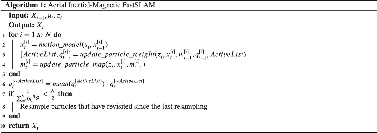
SLAM estimates a path and map concurrently. We present an extension of the FastSLAM algorithm used on a Roomba-style robot with a vector magnetometer by Vallivaara, Haverinen, Kemppainen, and Roning,15 shown in Algorithm 1, to the flight test dataset used by Canciani3 for aerial magnetic map-based navigation. Using identical measurement data, we achieve similar performance to the map-based method, despite starting off with no prior map. We modified the common FastSLAM algorithm to estimate INS errors and used them to correct an aircraft state estimate as illustrated in Figure 2. An INS produces a system state estimate. Then, FastSLAM uses scalar magnetometer observations and an INS error model to simultaneously estimate the drifting INS position errors and a magnetic anomaly map. Finally, the INS errors are removed from the original INS solution, resulting in a corrected whole state estimate, ie, INS Position Estimate + INS Position Errors = Corrected Position Estimate.

The system loosely couples an INS solution to magnetic intensity measurements to correct for state errors
While the concept of SLAM has been around since 198623 FastSLAM was first introduced by Montemerlo in 2003 as a factored solution to SLAM with unknown data association.24 Murphy25 first presented the factorization of the full SLAM posterior into a product of N+1 recursive estimators: one estimator over robot paths and N independent estimators over landmark positions, each conditioned on the path estimate
 1
1
This factorization can be efficiently approximated with a Rao-Blackwellized particle filter (RBPF), where each particle is a sample path of the vehicle. Each particle maintains its own hypothesized map and independently determines when it revisits a portion of its path. The general Bayesian recursion problem is solved here with a linearized dynamics model and nonlinear measurement equation from the marginalized particle filter paper by Schön, Gustafsson and Nordlund,26 specifically Algorithm I: Model 4. The error state variable x was partitioned into two horizontal position error particle states xn, and seven linearized error states xl: altitude, three-dimensional velocity, and three-dimensional tilt.
 2
2

The linearized Pinson error dynamics model F, described in Appendix A.1, was discretized at each time step to form the matrix A which was then partitioned into nonlinear and linear components for the linear dynamics model in Equations (4a) and (4b). The nonlinear measurement function which maps magnetic measurements to system states is represented in Equation (4c).
 3
3
 4a
4a
 4b
4b
 4c
4c
The strength of the driving noise is defined by Q, with 
 , and et = Ν (0, R). Q is defined in Appendix A.1.
The filter began with a known global position as assumed to be the case in the loss of GNSS availability. Particles were cast as potential aircraft paths based on the nine-state Pinson INS error model.27 Increasing inertial errors would eventually make the INS error model invalid but was not a problem in this instance due to the high-quality inertial system used over a relatively short time period. Longer flights could periodically apply INS feedback to keep the model valid. The propagation of particles approximated a proposal distribution of INS errors. When particles hypothesized path revisits, they interpolated expected intensities from a shared set of measurements conditioned to their individual paths, compared them to the current actual measurements, and were weighted using a Gaussian residual weighting function. Over time, particles with the most self-consistent magnetic intensity measurements at path revisits survived resampling to approximate the errors in the overall flight path. The INS solution was adjusted by the weighted sum of the particles’ position errors to provide a new position estimate. We will now describe each step of Algorithm 1 for a single time step. Central to understanding the algorithm is the concept of a revisiting particle. A particle is said to be a revisiting particle if that particle determines that it is nearby its own past trajectory. Note that each particle stores a hypothesized trajectory, and these trajectories, along with the magnetic measurements, create hypothesized magnetic maps. On line 2, the ith of N particles uses its previous state  and control input ut to propagate to its current state
  according to the nine-state Pinson INS error dynamics and noise model further described in the Appendix. On line 3, a particle compares its current state
  and measurement zt to its map model
  and returns an updated weight
  and list of currently revisiting particles, ActiveList. On line 4, a particle updates its individual map
  with the latest measurement
  and trajectory estimate zt. The weights of the particles that did not hypothesize a revisit are multiplied by the mean of particle weights on the ActiveList as shown in line 6. Line 8 states that if the number of effective particles falls below half of the total number of particles, systematic resampling occurs to replace poorly weighted particles with duplicates of highly weighted particles. The process concludes one iteration with an updated set of particles Xt approximating the current state estimate.
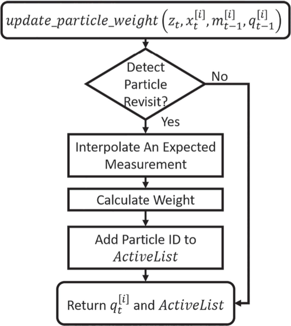
Our contributions primarily involve the particle weighting function in line 3 of Algorithm 1 and resampling in line 8. The update_particle_weight(·) function is further expanded with a flow chart in Figure 3. We will now step through each part of the process outlined in Figure 3.

Updating each particle weight depends on whether or not it hypothesizes a revisit
2.1 Detect particle revisit
Effectively detecting particle revisits was key to capturing spatial correlation from magnetic intensity measurements across time. A particle declared a path revisit when enough points from its previous trajectory lay within an experimentally tuned trigger radius. In defining a particle revisit, there were four primary considerations.
1. Choosing too small of a trigger radius creates false negatives. This makes a particle highly unlikely to ever detect previous discrete trajectory points which are spaced out as a function of data rate and vehicle motion.
2. Choosing too large of a trigger radius yields false positives. This does not provide a valid set of points to interpolate with and compare to current magnetic measurements.
3. Sequential weight updates for a particle during what is actually a single revisit event has a negative effect on filter performance.
4. Evaluating all particle’s proximity to all previous points in its trajectory scales poorly in computational cost over time without using a hierarchical data structure. We downsampled points to reduce computation time. This increased the effective distance between discrete data points in our particles’ paths and increased our required trigger radius.
2.2 Interpolate an expected measurement
Once a particle detected a path revisit, it selected a set of points s from its previous path and magnetic measurements from within a radius for interpolation as shown in Figure 4B. A sequence of the most recent values was ignored to prevent biasing the result of interpolation.15 Gaussian process regression (GPR) evaluated the interpolation point locations and associated magnetic measurements from the set of points s as a realization of a zero-mean multivariate Gaussian process.28 The GPR expected measurement function is written as follows:
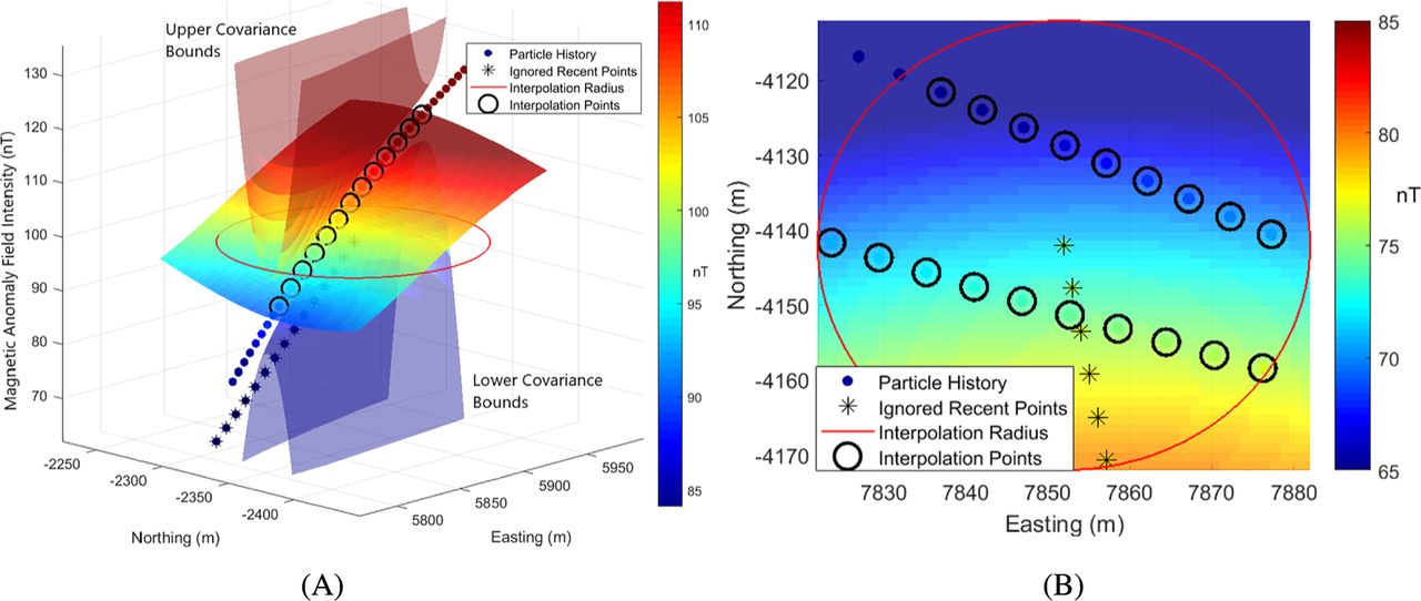
Gaussian process regression estimating a grid of points given some circled input points. A, GPR expected values and covariance around a line of points. B, GPR prediction around a set of scattered points
 5
5
GPR returned an expected value  for a query point, in this case, the ith particle’s current position
  , as well as a covariance
  at that point in time. The hyper-parameters σse, l, and σn were used in the squared exponential kernel function and were experimentally determined to be 50, 150, and 1, respectively. More research is required for possible uses of
  since the current filter used a tuned value of R = 102 for the weighting function (9) below. The function estimated
 6
6
where K, K∗, and K∗∗ were built by a squared exponential function as described by Ebden.28 The function to compute the individual cross terms between some x1 and x2 in K was
 7
7
GPR assumes a zero-mean multivariate Gaussian process. Therefore, a prior-mean correction was applied by removing the mean of the measurements of each particle’s interpolation points. Equation (6) becomes
 8
8
This method is illustrated in Figure 4A,B. Note that for a single line of past magnetic data as in Figure 4A, GPR simply fits the data to a plane—there is no information in the perpendicular direction of the trajectory. Contrast this to Figure 4B where there are two past trajectory lines yielding a more complex predicted field. Magnetic intensity scalar fields are guaranteed to be continuous. GPR has the benefit of modeling the field as a smooth best fit of measurements. As the filter interpolation area gets smaller, it approximately models a linear plane as visualized in Figure 4.
2.3 Calculate weight
Gaussian residual weighting evaluated the quality of a particle’s hypothesis by comparing the expected magnetic intensity with the actual measurement:
 9
9
where  was an active particle’s weight at the current time
  was the particle’s previous weight, zt was the current measurement,
  was the particle’s expected magnetic intensity from the measurement function h(·), and R was the filter measurement covariance term experimentally tuned to 100 nanoteslas. For both Vallivaara et al29 and the results seen here, an experimentally determined constant value of R for all particles returned better performance than the covariance value from GPR. The weighting of particles posed challenges when not all particles hypothesized revisiting at the same time. Vallivaara et al29 addressed this by weighting nonvisiting particles by the average weight of the visiting particles. We expanded on this by only resampling from particles which appeared on the ActiveList since the previous resampling step. Since information only entered the system during line revisits, this technique prevented the disproportionate favoring of particles which hypothesized many revisits over equally valid particles which were not revisiting as often. This change ended up being an essential factor in obtaining good algorithm performance.
2.4 Resampling
The standard particle filter criteria from Liu30 was used to determine when to resample:
 10
10
where N is the total number of particles. Importantly, only particles which appeared on the ActiveList since the previous resampling step were resampled.
3 FLIGHT TEST
A Cessna 208B like the one shown in Figure 5 collected magnetic intensity measurements, barometric altitude measurements, an unaided INS solution, and a GNSS-aided INS truth trajectory. This dataset was collected by Sander Geophysics Limited under United States Air Force contract in July of 2015.

Sander Geophysics Limited (SGL) Cessna 208B31
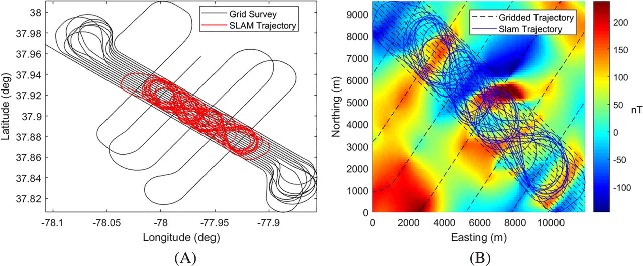
Two flight patterns were flown over a 9- by 12-km area, 150 m above ground level (AGL) in Louisa, Virginia as shown in Figure 6A. The first was a gridded survey to map the magnetic intensity field. The second was a looping flight pattern. These flights originally demonstrated map-based aerial magnetic navigation32 achieving 13-m distance root mean squared (DRMS) error over a 1-hour flight. The second flight’s many loops and path crossings made it a viable dataset to apply SLAM techniques. Figure 6B illustrates the magnetic anomaly intensity varying horizontally over the flight area.

Gridded and SLAM flight patterns. A, Flight patterns in latitude and longitude. B, Flight paths in relative horizontal distance over an interpolated magnetic anomaly field intensity
3.1 Isolating Earth’s magnetic anomaly field
The navigation signal used in this filter was created by perturbations in Earth’s core magnetic intensity field from magnetically susceptible crustal formations. Magnetic intensity measurements primarily include Earth’s core field, the crustal anomaly signal, aircraft disturbances, and temporally varying space weather effects known as diurnal magnetic variations.18
 11
11
The anomaly signal was approximated by removing the World Magnetic Model (WMM) core model, diurnal variations, and aircraft affects from the magnetic measurements. The WMM is produced by the US National Oceanic and Atmospheric Administration’s National Geophysical Data Center (NOAA/NGDC) and the British Geological Survey (BGS) as the standard model used for navigation, attitude, and heading referencing systems using the geomagnetic field. It is also used widely in civilian navigation and heading systems.33 Earth’s core magnetic intensity field was planar over the flight areas as the WMM shows in Figure 7A. Diurnal measurements observed at a separate ground station were recorded during the SLAM flight as shown in Figure 7B. Aircraft disturbance effects were determined through prior aircraft characterization by the geo-surveying company and are shown in Figure 7D. The crustal anomaly field provides the most spatial variation of the magnetic intensity field as shown by contrasting the WMM in Figure 7A, with the crustal field in Figure 7C. Note how the WMM is highly planar within this flight area, while the magnetic anomaly has much higher spatial frequency content.

Components of the magnetic intensity measurements. A, 2015 WMM model over the flight area. B, Diurnal variations during SLAM flight. C, Isolated magnetic anomaly field over flight area. D, Aircraft disturbance effects
3.2 Drifting INS state estimate
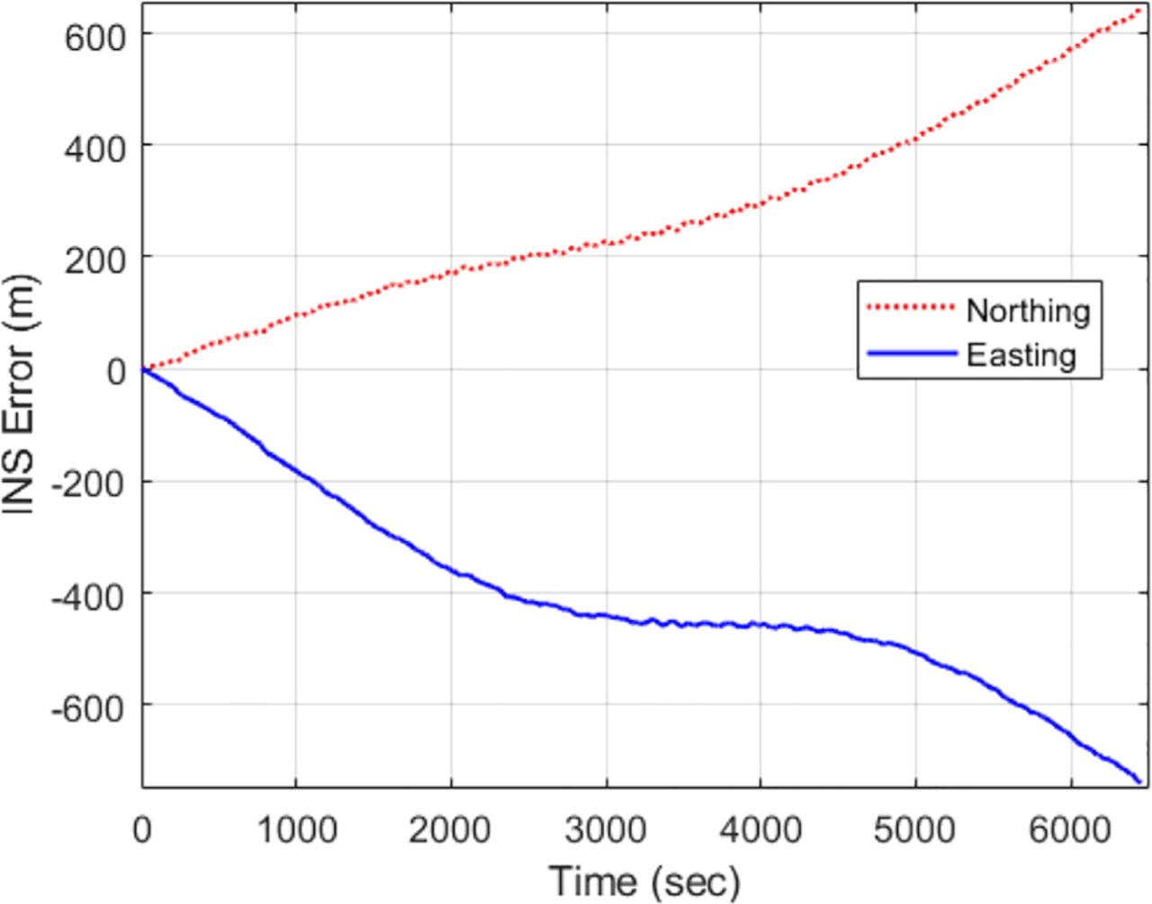
The INS measures the relative motion between the local vehicle body frame and the inertial reference frame. Vehicle dynamics are estimated by integrating measured acceleration and angular rate disturbances in the body frame and then transforming them to the local navigation frame to determine position and velocity estimates. Multiple integrations of measurement noise in the INS inevitably lead to a drifting navigation solution. State estimation uses linearized models to estimate the accumulating error states in the INS. The Pinson INS error model from Titterton and Weston27 was used to shape additive Gaussian white noise into angular and velocity random walk errors, which were coupled to form drifting horizontal and vertical position estimates. A navigation grade INS provided a real-time navigation solution. The drifting horizontal position errors in northing and easting components are shown in Figure 8.

Northing and easting drift of actual INS
4 RESULTS
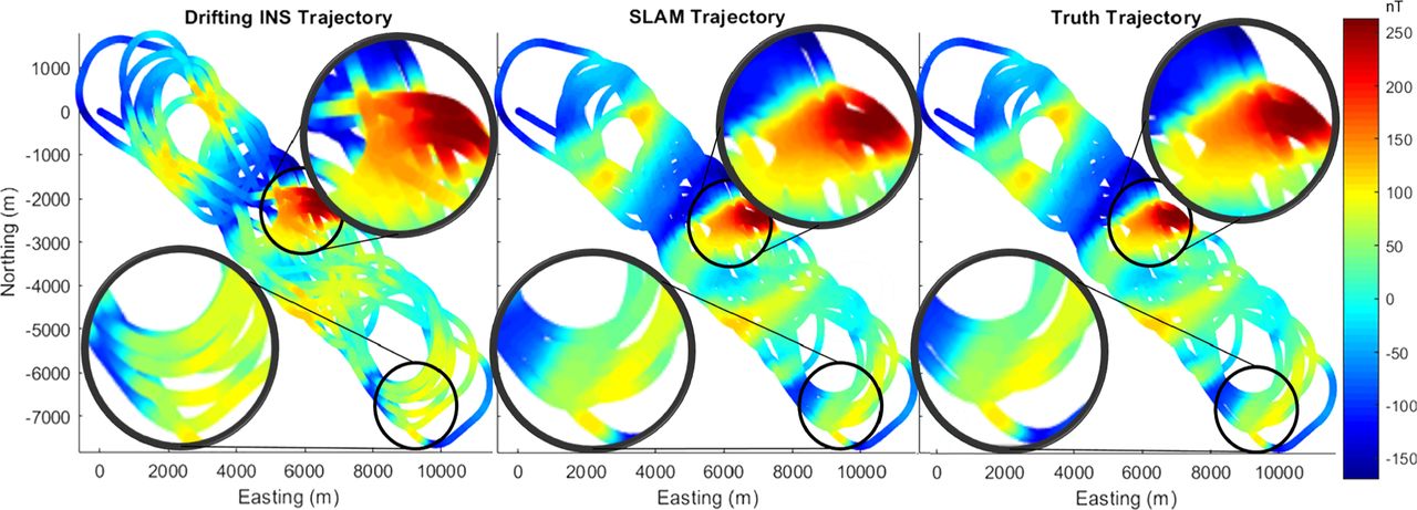
SLAM estimates a vehicle path and map concurrently. The filter performance can be illustrated in its ability to correct the magnetic map. The INS, filter, and truth trajectories are plotted in Figure 9. The colors correspond to the same set of magnetic intensity measurements with the mean removed. Comparing the INS estimate, SLAM solution, and GNSS truth trajectories overlaid with the same set of zero-mean magnetic intensity measurements illustrates how the position errors lead to measurement inconsistencies at path intersections. The drifting INS trajectory in Figure 9 has path crossings with different colors. This is clearly an error as there should be common magnetic measurements at common locations. Compare this to the SLAM or truth trajectory in Figure 9 and it is clear these maps are far more self-consistent. Although SLAM provides both a map and path estimate, this research focused on its navigation potential. The relative position error is defined here as the root mean square of the zero-mean filter error as written in Equation (12).

Comparing the INS estimate, SLAM estimate, and GPS truth trajectories overlaid with the same set of zero-mean magnetic intensity measurements emphasizes the correlation between position errors and measurement inconsistencies
 12
12
The filter converged to a relative position solution with a self-consistency of better than 20 m as seen in Table 1 and Figure 10. Table 1 compares the original error of the INS to the performance of the filter. Interestingly, the filter performed only 15% worse when using raw measurements uncompensated for aircraft effects or diurnal variation. This can be partly attributed to relatively minor magnetic disturbances from the specialized geo-surveying aircraft. Additionally, the short time span between revisiting trajectories relative to the time-varying components of diurnal variation and WMM fluctuation kept the actual magnetic field approximately time invariant for this flight. In other words, the spatial variation in the magnetic anomaly field dominated the time variant components of space weather effects over a short time span and the spatial variation from the WMM.
Filter performance after convergence

Filter errors and 1σ bounds using 1000 particles and R = 100. A, Northing position error. B, Easting position error. C, Euclidean distance error
It is interesting to note the uncertainty growing at the beginning of filter operation. This is due to the fact that single flight line crossings simply do not contain enough information to constrain the filter solution. As more and more flight lines cross their own past trajectories, stronger aiding information becomes available, and the filter uncertainty begins to decline. Note that these flights were conducted at only 150 m above ground level. The spatial variation in the magnetic anomaly field is greater nearer the crust and thereby has the best navigation potential. The real takeaway here is the similar performance to map-based aerial magnetic navigation without a map using SLAM techniques. An opportunity for improvement would be to incorporate a more realistic INS error model which includes accelerometer and gyroscope bias terms which are a significant source of INS drift. A better INS error model would represent a better proposal distribution and could provide a more accurate filter. There is significant potential for computational improvements as this research did not leverage the binary tree particle history structure of FastSLAM. It is also worth exploring graph-based methods, which have had promising results in WiFi SLAM.34
5 CONCLUSIONS
There are many research efforts to provide viable GNSS-alternative navigation methods. Magnetic navigation shows promise as one such method but is limited by the requirement for globally available and accurate magnetic maps. These maps greatly vary in quality and altitude. Fully sampled, low-altitude magnetic maps are expensive to create which presents barriers to using magnetic navigation on low-flying platforms such as UAVs. SLAM uses previous measurements and a revisiting trajectory to create a map and use it to navigate at the same time. This removes the dependency on a prior magnetic map for aerial magnetic navigation, especially for low-flying UAVs or in areas without magnetic maps. This paper introduced an RBPF that loosely coupled magnetic intensity measurements with an INS solution to constrain drifting errors to a relative position solution of tens of meters on real flight test data. This research has shown that the map dependency in aerial navigation can be removed by leveraging magnetic SLAM techniques common in robotics. Aerial magnetic SLAM is a powerful navigation technique that it is a globally available, passively sensed, and unjammable GNSS-alternative navigation method that does not require a prior magnetic map.
HOW TO CITE THIS ARTICLE
Lee TN, Canciani AJ. MagSLAM: Aerial simultaneous localization and mapping using Earth’s magnetic anomaly field. NAVIGATION. 2020;67:95–107. https://doi.org/10.1002/navi.352
AUTHOR CONTRIBUTIONS
The views expressed in this paper are those of the authors and do not reflect the official policy or position of the United States Air Force, Department of Defense, or US Government.
PRODUCT ENDORSEMENT DISCLAIMER
Reference herein to any specific commercial product, process, or service by trade name, trademark, manufacturer, or otherwise does not necessarily constitute or imply its endorsement, recommendation, or favor by the United States Government, the Department of Defense, or the Air Force Institute of Technology.
APPENDIX A: IMPLEMENTATION DETAILS
This appendix presents details pertaining to the INS error model and scalar magnetometer description.
A.1 Nine-state Pinson INS error model
Inertial navigation systems are used to measure the relative motion between a vehicle’s local body frame and an inertial reference frame. The dynamic motion of the vehicle can be determined by integrating acceleration and angular rate disturbances, correcting for Coriolis and gravitational effects, and then determining position and velocity estimates resolved in the local navigation frame. Twice-integrated accelerometer and gyroscope biases and noise inevitably lead to a navigation estimate that drifts over time. State space estimation models INS solution to estimate the whole state or the accumulating errors in the INS instead.
This section introduces a fundamental nine-state INS error model from Titterton and Weston.27
The generic nine-state Pinson error model states are x = [δp δv δɛ]T, where δp, δv, and δɛ are three-dimensional position, velocity, and tilt error vectors, respectively. The Pinson error model states propagate according to the linear dynamics equation  , where F is the linearized dynamics model and w is white Gaussian noise characterized by w ∼ Ν (0, Q). This F matrix can be broken up into nine submatrices relating position, velocity, and tilt errors to each other:
 A1
A1
The following notation described in Table A1 will remain consistent throughout the remainder of this section.
Pinson nomenclature
Titterton and Weston express north and east position errors in radians for latitude and longitude and vertical position error as positive upward altitude error,27 resulting in the following nine F submatrices:
 A2
A2
 A3
A3
 A4
A4
 A5
A5
 A6
A6
 A7
A7
 A8
A8
 A9
A9
 A10
A10
The model adds white Gaussian noise into the velocity and tilt states which are integrated which become random walk errors. The white noise strength is characterized by the matrix:
 A11
A11
A.2 Sensor description
Magnetic intensity measurements were collected with a self-oscillating split-beam Cesium-pumped vapor scalar magnetometer. These precision magnetometers are able to precisely resolve the intensity of a magnetic field with heading errors on the order of tenths of nanoteslas. A scalar magnetometer’s characteristics similar to the one used in the survey are listed in Table A2.
Scalar magnetometer characteristics
Footnotes
This article is a U.S. Government work and is in the public domain in the USA.
- Received March 19, 2019.
- Revision received December 12, 2019.
- Accepted December 30, 2019.
This is an open access article under the terms of the Creative Commons Attribution License, which permits use, distribution and reproduction in any medium, provided the original work is properly cited.


Jump to section
Related Articles
Cited By...
- No citing articles found.