

Abstract
The in-motion alignment for the underwater strapdown inertial navigation system is still a challenging problem due to various disturbances in the underwater environment. In this paper, a novel in-motion alignment method, based on the Lie group representation, is developed. In this method, the process model is rewritten using the Lie group of the constant attitude matrix between two inertial frames as the state. An exact linear measurement model is constructed by analyzing the effect of the sensor errors in calculating the velocity vector. Next, the state-dependent Lie group filter is designed basing on accurate derivation expressions for the covariance matrices of state-dependent noises. The simulation and experiment results demonstrate that the proposed method can achieve better alignment accuracy and time than the existing method. The accuracy improves by 70% with the quaternion Kalman filter.
1 INTRODUCTION
Strapdown inertial navigation system (SINS) is a useful navigation system with lower cost, reduced size, and better reliability than other navigation systems, e.g., Platform Inertial Navigation, GNSS (Global Navigation Satellite System), or SLAM (Simultaneous Localization and Mapping). For SINS, the initial attitude alignment is a critical prenavigation process. During the initial alignment process, the attitude matrix between the body frame and navigation frame is determined based on measurement information from inertial sensors. Existing methods are usually performed in stationary mode (Fang & Wan, 1996; Wang & Shen, 2005); however, for some specific conditions, such as underwater, in-mooring, and in-flight, in-motion alignment is essential (Cui, Mei, Qin, Yan, & Fu, 2017; Emami & Taban, 2018; Li, Wu, Wang, & Lu, 2013). There are many factors that make underwater vehicle attitude alignment challenging. The main two factors are: the GPS-aided sensors may be affected by disturbances or not available, and in-motion alignment might be continuously implemented because the vehicle may remain in motion due to water flow (Ben, Zhu, Li, & Wu, 2011).
Over the last decade, alignment methods based on the tracing gravity drift in the inertial frame for the in-motion SINS alignment have received attractive attentions. Because the projecting velocity in an inertial frame can be separated into acceleration and angular measurements, alignment methods that trace the velocity of apparent motion in the inertial frame can effectively solve the in-motion alignment problem. The inertial frame alignment methods can be divided into two categories according to the different features in the construction of the vector of observations and the calculation procedure of the alignment matrix. These two methods are the dual-vector attitude determination one and the attitude-optimization-based one. In the former one, the initial attitude matrix is determined by selecting the apparent gravitational motion vectors at two different moments, in which the projections in the initial inertial navigation frame are given as non-collinear vectors (Li et al., 2013; Li, Ben, & Sun, 2013; Liu et al., 2015; Liu, Zhao, Liu, & Wang, 2015; Qin, Zhu, Zhao, & Bai, 2008; Yan, Bai, Weng, & Qin, 2011). To improve alignment accuracy, velocity vectors integrated by gravitational acceleration instead of gravity vectors are used in an improved alignment solution (Li et al., 2013; Liu et al., 2015; Liu, Zhao, Liu, & Wang, 2015). These self-alignment methods are applicable to mooring alignment; thus, the rotation of the Earth from the gyro measurement is not required to be separated. However, in these methods, a long alignment time (more than 300 seconds) is required to ensure sufficient random noise smoothing and time intervals between two vectors to avoid collinearity and ensure solution accuracy with the dual-vector method. The second method is attitude-optimization-based initial alignment, which transforms the initial alignment problem into a continuous attitude determination problem by using infinite vector observations (Ben et al., 2011; Chang, Li, & Chen, 2015; Kang, Fang, & Wang, 2013; Kang, Ye, & Song, 2014; Li, Tang, Lu, & Wu, 2013; Wu & Pan, 2013; Wu, Wu, Hu, & Hu, 2011; Zhou, Qin, Zhang, & Cheng, 2012). All these methods listed in these papers are based on the decomposition of the attitude matrix into earth motion, inertial rate, and alignment matrix, but have different vector observation constructions and alignment matrix calculation procedures. For underwater alignment, the vector observation is usually constructed based on the velocity integration formula in the body frame because of the adoption of the Doppler Velocity Log (DVL), which is a common auxiliary tool for underwater navigation and provides velocity measurement in the body frame. The least-squares approach (Kang et al., 2014; Li et al., 2013) and the Kalman filtering approach (Zhou et al., 2012) are used to estimate the alignment attitude matrix. In Zhou et al. (2012), a special measurement equation resulting in a linear pseudo-measurement equation is constructed and a novel quaternion Kalman filter is proposed to estimate the attitude quaternion.
The attitude-optimization-based initial alignment method is superior to the dual-vector attitude determination method in alignment accuracy and alignment speed (Liu, Zhao, Liu, & Wang, 2015). However, there are inherent flaws in this alignment method because unit quaternion is used to represent the rigid-body attitude. In this method, there is a double coverage of the set of attitude spaces in the sense that each attitude corresponds to two different quaternion vectors. This implies that the closed-loop properties derived using quaternions may not hold for the dynamics of the physical rigid-body on SO(3) × ℜ3. Therefore, an attitude-optimization-based initial alignment method using the unit quaternion representation may yield undesirable unwinding phenomena during the alignment process. Meanwhile, a nonlinear filter must be applied in the attitude-optimization-based initial alignment method because the measurement model is a nonlinear equation for quaternion vector measurements (Chang et al., 2015). Although a linear pseudo-measurement equation is constructed via mathematical transformation of quaternion matrices to solve this problem (Zhou et al., 2012), the zero-measurement value induces an all-zero state value, which causes the filter to converge slowly (or even diverge).
The special orthogonal matrix (SO(3) × ℜ3) is global and unique in the sense that each physical rigid-body attitude corresponds to exactly one rotation matrix. Additionally, rigid-body rotation space SO(3) × ℜ3 is a Lie group (Chaturvedi, Sanyal, & Mcclamroch, 2011), which is compact and contains the full attitude of the rigid-body. Thus, much effort has been paid to the development of attitude representation and estimation using a Lie group (Barrau & Bonnabel, 2015; De Ruiter, 2014; Markley, 2006; Saccon, Trumpf, Mahony, & Pedro Aguiar, 2016). Motivated by above observations, this paper is going to develop a novel in-motion alignment method for underwater vehicle applications using a Lie group to represent the attitude. Based on the concept of attitude matrix decomposition, the attitude change matrix of the body frame and the navigation frame and the constant matrix between two inertial frames are reformulated using Lie group representation. Then, the state equation, which uses the Lie group of the constant matrix between two inertial frames as the state vector, is constructed. The linear measurement equation using Lie group representation is also constructed using a pair of velocity vectors in two solidification inertial coordinate systems. Because the special state vector is a Lie group, a state-dependent Lie group filter is developed to solve the attitude matrix estimation problems. In addition, because the measurement noise is dependent on the Lie group, an important contribution of this paper is to analyze and calculate the covariance matrix of this state-dependent measurement noise. The existing general expressions for the covariance matrices of this state-dependent noise are extended from the vector form to the Lie group representation. Then, the covariance matrix of the Lie-group-dependent noise is calculated according to the mapping relationship between the Lie group and the Lie algebra. The simulation results show that this in-motion alignment scheme can effectively solve the alignment problem of SINS in the underwater environment.
The rest of this paper is organized as follows. In Section 2, we compare existing attitude representation methods and introduce the basic concepts related to Lie groups. In Section 3, based on the aided velocity in the carrier frame, the system model is established and described in a Lie group representation. Section 4 presents the Lie group filter with state-dependent noise and analyzes the measurement noise covariance matrix. Simulations are presented in Section 5, followed by which the conclusions are drawn.
1.1 Coordinate system definitions
Several coordinate frames that are used in the alignment of SINS in an inertial system are listed as follows:
The n frame is artificially selected as the ideal navigation frame with east-north-up axes.
The b frame is the body-fixed frame of the sensor.
The e frame is the Earth-fixed frame.
The i frame is the inertial coordinate frame.
The n0 frame is the inertial coordinate frame obtained by fixing the n frame at the initial time.
The b0 frame is the inertial coordinate frame obtained by fixing the b frame at the initial time.
2 LIE GROUP REPRESENTATION FOR RIGID-BODY ATTITUDE
2.1 Comparison of existing attitude representation methods
A rigid-body attitude is usually represented by three or four parameters. Three-parameter representations of the attitude include Euler angles, Rodrigues parameters, and modified Rodrigues parameters. Euler angles are singular in kinematics because the transition from the time rate to the angular velocity vector is not globally defined. Rodrigues parameters and modified Rodrigues parameters are also geometrically singular because they are not defined for 180° of rotation (Zhou et al., 2012). Four-parameter representations of the attitude include unit quaternions and axis angles. Since the four-parameter representations of the attitude are global and are free of the singularity problem, thus they are typically adopted in practical applications.
The unit quaternion representation of attitude is the most common four-parameter representation used in attitude control and determination because its two attractive features, a linear dynamic equation and a nonsingular formulation. However, the map from the space S3 of the unit quaternions to the space SO(3) × ℜ3 of the rotations is a double coverage map, and each corresponding rule governing attitude behavior is represented by a pair of opposite unit quaternions ±q. One implication of this non-uniqueness representation is that the closed-loop properties derived using quaternions may not hold for the dynamics of the physical rigid-body in SO(3) × ℜ3 (Zhou et al., 2012). Therefore, the gradual and stable equilibrium of the quaternion does not guarantee the gradual stabilization of the posture. If the non-uniqueness of the unit quaternion representation is neglected, the quaternion may not hold for the physical rigid-body, and quaternion-based methods may yield undesirable unwinding phenomena in the process of attitude control and determination. Figure 1 shows the projection from the quaternion space to the physical rotation space.
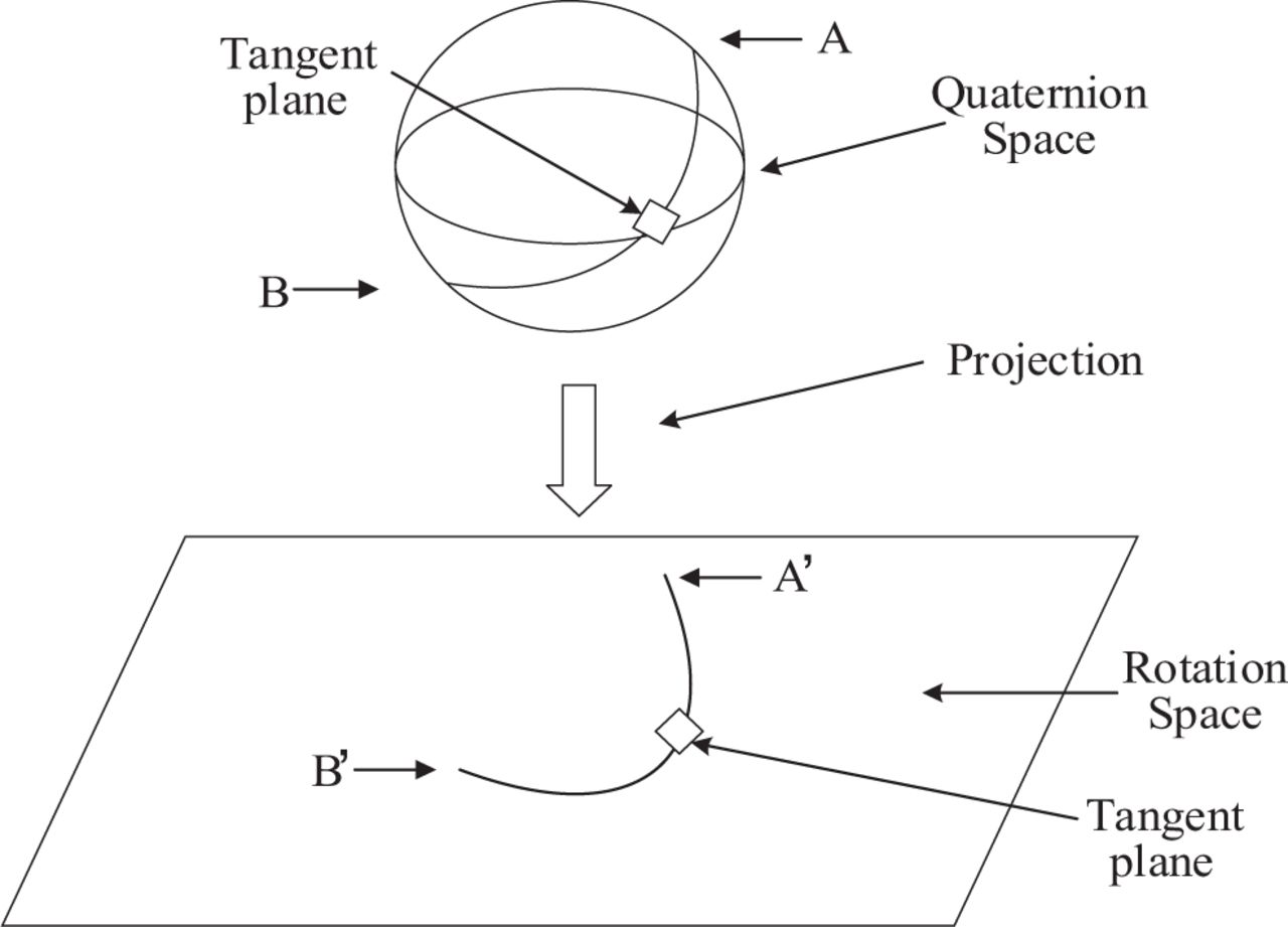
Projection from quaternion space to physical rotation space
2.2 The basics of Lie group representation
A Lie group is a group G that is a smooth manifold and for which the group operations (g, h) → gh and g → g−1 are smooth. A Lie group is abelian if gh = hg for all g, h ∈ G (Markley, 2006). The special orthogonal group SO(3) × ℜ3 is a subgroup of the general linear group GL(n), and the set of this special orthogonal group is defined as
 1
1
with an associated Lie algebra, which is a set of 3 × 3 skew-symmetric matrices, given by
 2
2
The function [⋅]× denotes a map from a 3 × 1 vector to its corresponding 3 × 3 skew-symmetric matrix. For any k ∈ ℝ3,
 3
3
The inverse function is [⋅]∨ ∶ so(3) → k, k ∈ ℜ3.
Given R(t) ∈ SO(3), if the matrix  is skew-symmetric (Markley, 2006), then
 4
4
where  . For a given sampling time interval T, the discrete implementation of the differential equation is
 5
5
The matrix exponential that maps so(3) onto SO(3) is well known and can be derived from Rodrigues’ equation for rotations:
 6
6
The initial alignment problem can be understood as the problem of determining the attitude matrix between the carrier coordinate system and the navigation coordinate system. Because the vectors in the attitude matrix A for SINS are orthogonal, thus this attitude matrix has the following properties:
 7
7
3 INITIAL ALIGNMENT USING THE QUATERNION REPRESENTATION
According to the attitude matrix chain rule, the matrix for the attitude transformation from the body frame to the navigation frame can be decomposed into three separate attitude matrices, namely, an Earth motion matrix, an inertial rate matrix, and an alignment matrix. The initial attitude matrix is thus written as a product of three continuous rotation matrices:
 8
8
where  denotes the rotation matrix from coordinate system A to coordinate system B and n(0) and b(0) denote the initial inertial coordinate systems n and b, respectively. Therefore,
  can be rewritten as the following equations:
 9
9
 10
10
where  represents the angular velocity vector of coordinate system A relative to coordinate system B; in coordinate system B and
  is slowly changing with the movement of the vehicle. The value of
  is unknown if the current position is unavailable; however, it is a small value that can be neglected. Consider that
  , where
  is the measurement from the gyroscope.
  and
and  are initially equal to the identity matrix. Then, Lie groups
  and
and  can be rewritten as Equations (9) and (10) in each step. Given an estimate of the rotation matrix
  , the attitude matrix can be obtained based on Equation (8). Furthermore, the current location information Pn(tk+1) can be obtained by using Equation (11):
 11
11
For underwater alignment, since the aided velocity obtained from the DVL is expressed in the body frame, it is unlikely for an autonomous underwater vehicle (AUV) to move a large distance in a short time. The traditional method is to use the velocity differential equation in the body frame to build the dynamics model. The Earth’s rotation and the movement of the navigation frame relative to the Earth’s frame are ignored when building the model. In this paper, to reflect the influence of the Earth’s rotation, an inertial force equation is constructed in the b0 frame, which makes the model more accurate:
 12
12
where v represents the velocity, f represents the specific force, and g represents the acceleration due to gravity. The velocity in the b0 frame can be determined using the DVL measurement and the velocity induced by the Earth’s rotation in the navigation frame and is given as
 13
13
where  , with r being the Earth’s radius and L being the local latitude.
Integrating both sides of Equation (12) and substituting Equation (13) into the result, we obtain
 14
14
After a rearrangement, Equation (14) becomes
 15
15
Then, the formula for  is
is
 16
16
where
 17
17
 18
18
The sampling time for the gyroscope and accelerometer is chosen to be a fixed value. Thus, α(t) and β(t) can be accurately calculated using a suitable numerical algorithm. The calculation of β(t) is given as follows:
 19
19
Then, one has that
 20
20
Because the values used to calculate β(tk) are constants that can be found in a reference table, β(tk) is considered to be a precise measurement. Moreover, α(tk) is calculated as follows:
 21
21
Based on the quaternion representation, Equation (16) can be further written as
 22
22
where  denotes the quaternion representation of
  and ⊗ denotes quaternion multiplication.
Using Equations (8) and (22), many studies have investigated in-motion alignment methods based on continuous attitude determination via the q-method approach and the Kalman filtering approach. The q-method approach can yield a closed-form optimal estimation of the quaternion while explicitly preserving the unit-norm property.
It is obvious that Equation (22) is a nonlinear equation for the unit quaternion representation. Therefore, main filtering approaches used to estimate the sequential quaternion in attitude-optimization-based initial alignment methods are based on nonlinear filters. In Zhou et al. (2012), quaternion Kalman filter (QKF) approach was developed to estimate the attitude quaternion by constructing a special measurement equation called the linear pseudo-measurement equation.
First, Equation (22) is multiplied by  from the right on both sides and transposed:
 23
23
Then, the alignment model can be written as
 24
24
Based on the results in Kang, Ye, and Song (2014), the form of Hamiltonian operator in the Clifford algebra can be defined as:
 25
25
 26
26
Then, the quaternion product can be written as
 27
27
 28
28
Combining Equations (27) and (28) together, the measurement equation for the QKF can be written as:
 29
29
The measurement matrix H can then be defined as
 30
30
 31
31
 32
32
4 INITIAL ALIGNMENT USING A STATE-DEPENDENT LIE GROUP FILTER
Though the alignment methods are attractive and effective, there are still some flaws in these methods. In these methods, a nonlinear filter operates on a nonlinear quaternion measurement model. Although the QKF was developed to estimate the attitude quaternion by constructing a linear pseudo-measurement equation, it weakens the convergence speed and also reduces the accuracy when the left-hand side of the measurement equation is zero. Moreover, all existing initial alignment methods estimate quantities other than the attitude quaternion, such as the sensor errors (bias, scale factor, etc.). Because the sensor measurements are directly used to calculate α and β, the alignment accuracy is easily disturbed by sensor error, especially noise from accelerometers and gyroscopes.
To overcome these flaws of the quaternion representation, a Lie group representation is used to replace quaternion representation in the alignment process to improve the initial alignment performance in our proposed method. In this section, the basic attitude formula is constructed based on the differential equation for Lie group, and a linear measurement model is structured based on the Lie group representation. Then, a relatively accurate sensor noise analysis is presented for constructing the new measurement model. To overcome the problem of state-dependent measurement noise, a novel state-dependent Lie group filter is developed for estimating the initial attitude.
4.1 Initial alignment model using Lie group filter
According to Section 2, all rotation matrices can be represented using the Lie group representation. Therefore, we can rewrite Equations (9) and (10) using the differential equations for the Lie group:
 33
33
 34
34
where R ∈ SO(3) represents the Lie group. These equations can be solved by Equation (5).
Then, Equation (8) can be further rewritten as
 35
35
where  is the Lie group used to represent the rotation matrix at the initial instant.
From Equation (21), the calculation of α(tk) uses gyroscope and accelerometer measurements; thus, sensor error is the major source of disturbance noise for α(tk). These errors will eventually lead to the uncertainty measurement noise in the measurement model. Discernible estimation errors cannot be avoided, and the performance will be deteriorated if the measurement covariance matrix adopted in the Kalman filter is unable to detect and track the real changes in measurement noise.
To analyze the effects of sensor error and to construct a precise alignment model, the sensor errors will be taken into account in α(tk). Let εg and εα denote the gyroscope random error and the accelerometer random error, respectively. Adding the random sensor errors into the last term of Equation (18) gives that
 36
36
From Equation (36), it yields that
 37
37
Merging Equations (21) and (36) together, we obtain
 38
38
where
 39
39
 40
40
 41
41
Based on the above analysis, the final representation of  with random sensor error is given as
 42
42
If the sampling period is short, we can use the linear forms of the angular rate and acceleration:
 43
43
 44
44
Integrating the angular velocity, the incremental angle can be obtained as:
 45
45
 46
46
From the above formulas, we have
 47
47
 48
48
Similarly, one can get that
 49
49
 50
50
Using Equations (20) and (21), β(tk) and α(tk) can be calculated in each sampling period, however, finding the optimal estimation  is a problem. The proposed Lie group filter significantly contributes to the solution of this problem. Consider a state variable X that represents
  , which is a constant matrix. The discretized system model is constructed as
 51
51
 52
52
where X ∈ SO(3), βk+1, and αk+1 are two 3 × 1 vectors that are calculated using Equations (20) and (21), respectively, at tk+1. The vector βk+1 is obtained using the Earth’s rotation rate  and the component of gravitational acceleration in the navigation frame (gn), both of which are known. Clearly, these values are just relatively accurate as αk+1 contains a variety of sensor measurements (e.g.,
  is measured via a gyroscope and fb is measured via an accelerometer). The coupled measurement noise, denoted by δαk+1, is defined as
 53
53
where αk+1 is the exact value of the observation.
4.2 Analysis and design of the state-dependent noise covariance matrix
The above discretized system model can be solved using a Lie group filter. However, using the traditional measurement noise covariance matrix for state-dependent measurement noise may lead to imprecise estimation. In this section, based on the definition of the noise covariance matrix, the difficulty of using the traditional measurement noise covariance matrix for state-dependent measurement noise is explained subsequently. Because the noise and the state are linear and independent, a second term is developed to construct an exact expression for the state-dependent measurement noise covariance matrix. The state error and covariance matrix are defined based on the Lie group representation, and the propagation equation is given. Then, a novel Lie group filter is presented.
For simplicity, the measurement equation is rewritten as
 54
54
where
 55
55
Suppose that δαk+1 is the sum of two white Gaussian noise components with covariance matrix Rk+1 = (σ1 + σ2) I3. E{δαk+1} = 0 is statistically independent of the state Xk+1. In the usual Kalman filter framework, the mean value of Vk+1 is approximated to be zero, i.e., E{Xk+1δαk+1} = 0, where Xk+1 is the ideal value of the state. The state-dependent measurement noise covariance matrix is expressed as
 56
56
In the actual filtering process, Xk+1 is an unknown, and the state estimation  is used instead of Xk+1. In practical applications, Vk+1 is defined as
 57
57
where  denotes the estimated value of the state at tk+1. The error between Xk+1 and
  leads to inaccuracy of the covariance matrix of Vk+1. It is supposed that
  , where u characterizes the error between
  and X. Then, the real representation of the covariance matrix of V is given as
 58
58
Clearly, this matrix can be further split into two parts:
 59
59
A more concise representation of Equation (58) is expressed as
 60
60
The second term in Equation (60) is a matrix representation associated with the state and measurement noise, arising from the state-dependent measurement noise. Motivated by a theory similar to the one that applied to vector state-dependent noise in Alexander (2008), an extended theory based on the Lie group representation is presented in this paper. A more precise expression will be proposed in this section, and the relationship between the state error and measurement noise will be revealed to develop the second term.
Because Vk+1 represents state-dependent measurement noise, an exact expression for its covariance matrix is derived to design the filter. A similar and general form of the state-dependent noise covariance matrix is provided in the proposition presented in the appendix. These general results are applied to our special case, and the measurement equation is addressed in a similar way.  denotes the estimated value at tk+1. ξk+1 is the estimated state error of a Lie group that has a mapping relation with SO(3) (as discussed in the next section). The covariance matrices of ξk+1 and Vk+1 are Pk+1 and
  , respectively. δαk+1 and ξk+1 are independent. Under the assumption that δαk+1 is a white Gaussian noise with covariance matrix Rk+1,
  can be expressed as
 61
61
where  is the predicted value of Xk+1 and ⊗ is the Kronecker product. The matrix
  is defined as
 62
62
with
 63
63
The vectors ei, i = 1,2,3 are the standard basis vectors in ℜ3. The exact expression for  has a unique form given in the proposition in the appendix.
The first term on the right-hand side of Equation (61) is the usual approximation of the state-dependent measurement noise covariance matrix in the Kalman filter framework. The second term incorporates the error  into the expression. This term includes the product of δαk+1 and the error
  . The expression is derived by considering the linearity of the state-dependent noise with respect to Xk+1, which makes the filtering process more accurate.
4.3 Lie group filtering process
Compared to the traditional Kalman filter, the proposed filter directly estimates the rotation matrix instead of the state vector. Due to the properties of the special observer for a Lie group, the group multiplication operation (rather than addition) is proposed for updating the state value. The prediction and updating steps are performed as follows:
 64
64
 65
65
where Υ(⋅) is a function mapping ℜ3 to ℜ3×3 on a Lie group. The link between the proposed updating step and the traditional step can be understood in this way. The estimation error  is defined on ℜ3×3. According to the left-right equivariance hypothesis,
  can be interpreted as a Lie group equivalent to
  .
.
In fact, the defined invariant output errors represent a transformation from a linear error to a multiplicative group, which is an isomorphic transformation.
 66
66
 67
67
In the process of applying the proposed filter, the mean square error matrix P is derived from the estimation error. Thus, the error variables ηk+1 and ηk+1/k are obtained through the Markov process. The certification process is given as follows.
Substituting Equations (65) into (67), we obtain
 68
68
Therefore, ηk+1 and ηk+1/k can be rewritten as
 69
69
 70
70
Because βk+1 and αk+1 are calculated at regular intervals of time, the gain function Υ can be tuned freely. Analogous to the gain in the Kalman filter, the gain function Υ can be structured in the following way. Because the error state and model noise are relatively small, an exponential map is used as a projection of the Lie algebra of the group. Let χ → exp([χ]×) denote the exponential map, for which the specific calculation process has been given. Its inverse function is defined as R → log([R]∨). The state error is defined as
 71
71
 72
72
The innovation of the Lie group filter is defined as
 73
73
and the gain function is given as
 74
74
Then, the new definition of the state error is
 75
75
 76
76
Here, to simplify the calculation, we consider only the first order of the exponential expansion, ([χ]×) ≈ I3 + [χ]×:
 77
77
 78
78
Here,  .
.
If the error variance of the state is defined as P = E{ξξT}, then the gain Kk+1 can be obtained using the traditional Kalman method. First, a priori error covariance of the state is computed:
 79
79
where Φ is a 3 × 3 identity matrix and
 80
80
 81
81
 82
82
Sk is the mean square deviation of the innovation, which describes the influence of the state and noise on the filter gain. In the Lie group filter, the rotation matrix is directly selected as a state matrix. In new forms of the state error, the innovation and the measurement matrix based on the Lie group representation, which take advantage of the unique nature of the Lie group and the mapping relation between the Lie group and Lie algebra, are innovatively defined. An exponential mapping function is employed to correct the a priori estimation with the innovation. The propagation result is similar to that of the Kalman filter, which aims to estimate the minimum variance of the state error.
The Lie group filtering algorithm is proposed as follows:
Filter initialization: X0 = I3 and P0 = 5I3.
Filtering process:
 83
83
 84
84
 85
85
 86
86
 87
87
 88
88
 89
89
 90
90
The process of initial alignment is summarized as follows:
Step 1: Initialize
 and .
and .Step 2: When the gyro and acceleration information are available, update
and using Equation (33) and part of Equation (34).Step 3: When the aided velocity in the b frame measured by the DVL is available, update α(tk) and β(tk) using Equations (20) and (21).
Step 4: Use the proposed Lie group filter estimation
to update the attitude transformation matrix according to Equation (35) and the current geographic position Pn by Equation (11).Step 5: Return to step 2 unless the end of the initial alignment phase has been reached.


5 SIMULATIONS AND EXPERIMENTS
In this section, a simulation model of underwater vehicle motion is designed to verify the effectiveness of the proposed alignment method. The pitch, roll, and yaw are supposed to conform to cosine change, which are adopted to simulate the effects of water flow around underwater vehicles. Yaw ψ, pitch θ, and roll γ represent cyclical changes. The model of an AUV’s attitude is described as
 91
91
 92
92
 93
93
where Ay, Ar, Ap are the amplitudes of three attitude angles; ωy, ωr, ωp are the angular velocity; ϕy, ϕr, ϕp are initial phases; and ψ′ is the initial azimuth.
The line speed is set to less than 3 m/s, and described as
 94
94
where i = x,y,z, ADi is the amplitude of speed; ωDi is the frequency of speed; ϕDi is the initial phase.
The initial position is at 116° east longitude and 38° north latitude. The random drift of the gyro is 0.01°/h, the random travel coefficient of the gyroscope is  , the constant deviation of the accelerometer is 1 × 10⁻⁴g, the standard accelerometer measurement white noise is 1 × 10⁻⁵g, the DVL bias is 0.5% of the voyage velocity, and the sampling frequency of the DVL is 1 Hz.
5.1 Simulation results and analysis
Case 1: The amplitudes of wind and wave are small, the initial azimuth is 30°, and parameters of attitude angles and speed are listed in Table 1 (Tal, Klein, & Katz, 2017).
View this table:TABLE 1General condition
Case 2: The amplitudes of wind and wave are big, the initial azimuth is 120°, and parameters of attitude angles and speed are listed in Table 2 (Kang et al., 2014).
View this table:TABLE 2High wave amplitudes
Case 3: The influence of undercurrent will be simulated. The AUV moves in a circle and rotates around itself (Liu, Wang, Deng, & Fu, 2017).
 95
95
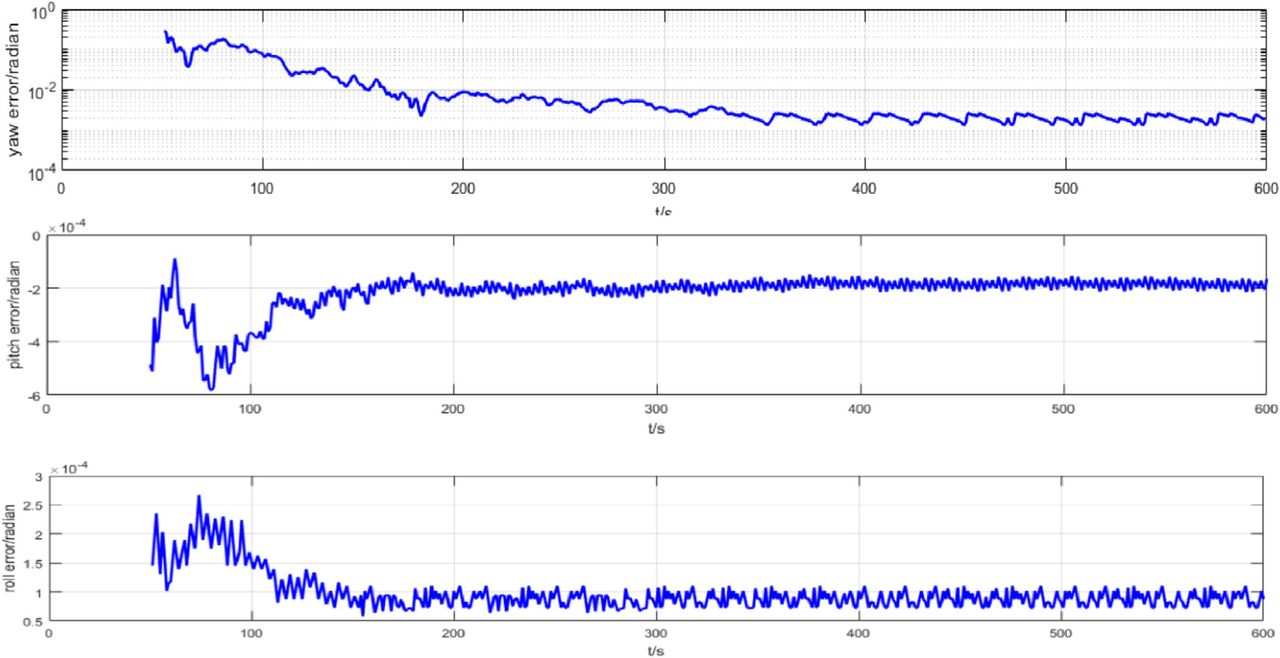
The proposed filter, called state-dependent Lie group filter (SLGF), runs for 600s. In order to display the alignment results clearly, Figures 2–4 display the attitude errors in three axes from 50s to 600s, and the attitude errors from 0s to 50s are not displayed. The yaw, pitch, and roll errors are reduced to 5.818 × 10⁻³, 1.45 × 10⁻⁴, and 5.82 × 10⁻⁵ after 200s in Case 1 and reduced to 6.69 × 10⁻³, 1.745 × 10⁻⁴, and 5.818 × 10⁻⁵ after 200s in Cases 2 and 3. From these figures, the robustness and the anti-interference ability of the proposed SLGF has been verified. The simulation shows that the proposed alignment method can achieve better convergence speed and high accuracy, which indicates that the SLGF has a great robustness in various conditions. In addition, the convergence speed of the three attitude angles is equivalent.

Initial alignment simulation results under general condition

Initial alignment simulation results under high wave amplitudes condition

Initial alignment simulation results under undercurrent effect
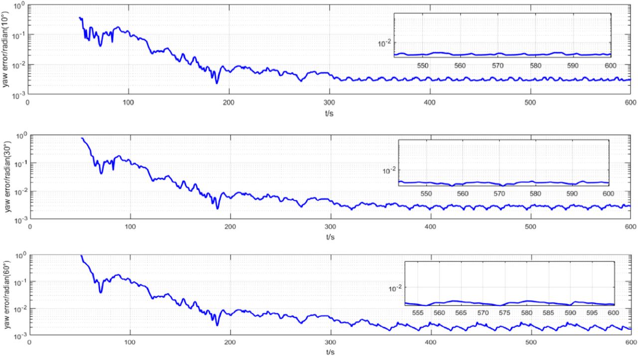
In Figure 5, the values in Table 1 are taken and various misalignment angles are chosen to prove the convergence. As seen in the figure, the errors for various misalignment angles converge over time, though there is oscillation before 100s. The smaller the misalignment angle, the more pronounced the oscillation. The alignment accuracy is higher with the reduction of the misalignment angle. When the initial error angles are 60°, 30°, and 10°, the final alignment accuracy is approximately 1.16 × 10⁻³, 5.8×10⁻⁴, and 2.9×10⁻⁴, respectively.

Yaw errors for various misalignment angles
5.2 Experiment results and analysis
The AUV is affected by external forces such as wind, engine rotation, wave surging, and other complex disturbances, which make its movement very uncertain. When the AUV is affected by water disturbances, its alignment time will be longer, and the alignment accuracy can significantly reduce. Due to limitations of our experimental capabilities, we use a low-speed ground vehicle to simulate motion conditions of the AUV. In this case, the alignment accuracy is affected by the motion dynamics including effects such as engine vibrations, road bumps, and vehicles’ acceleration/deceleration. These non-constant velocity components of the ground vehicle motion can mimic non-static conditions of the AUV to some extent.
We conducted an experiment at Beijing University of Technology. Experiments were implemented using the XW-ADU7612 attitude azimuth integrated navigation system, which is presented in Figure 6. XW-ADU7612 has a built-in inertial measurement unit and a dual GPS. Through an improved integrated navigation and attitude measurement algorithm, XW-ADU7612 can output a high-precision attitude angle that was used as a reference. By comparing the attitude angle obtained by various alignment methods and the attitude angle measured by XW-ADU7612, we can verify the advantage of the proposed method. Table 3 shows the azimuth precision of XW-ADU7612. In the experiment, we used the odometer to provide the velocity as the auxiliary information. The principle of the odometer is to obtain the circumference by measuring the number of turns of the wheel, and then the speed can be calculated. Thus, the odometer measures the speed of the body frame (b frame). DVL is an instrument that measures velocity based on the Doppler effect of sound waves in the water. Therefore, DVL measures the speed of the b frame as well. Although the odometer-based velocity accuracy is not as good as DVL, it can be used to verify advantages and disadvantages of various attitude estimation methods. In this experiment, Crossbow VG700AB is used for the system under test. The precision of IMU and the odometer is presented in Table 4. The trajectory of the car is shown in Figure 6.
System precision of IMU and odometer
System precision of XW-ADU7612

Installation diagram of experimental facilities and trajectory figure
Figure 7 compares the SLGF results with the quaternion Kalman filter (QKF), the singular value decomposition (SVD), and the Lie group filter (LGF) without the reconstructed noise covariance matrix, which is taken from our previous work. We adopt the logarithmic scale for angles and the linear scale for the time to draw the experiment figure. Because of the logarithmic scale, Figure 7 shows only those parts where the error is greater than zero. The analysis of the variance and mean of the last 100s data under different methods are shown in Table 5. We also present standard deviation for the steady-state region in Table 6.

Compare with other methods
Attitude angle error analysis
Standard deviation for the steady-state region
From Figure 7, QKF, LGF, SVD, and SLGF all converge over time, but LGF and SLGF have a better performance than QKF and SVD. As shown in Tables 5 and 6, the attitude angle error and the standard deviation of SLGF and LGF is much smaller than QKF and SVD. Meanwhile, from Figure 7 and Tables 5 and 6, it can be seen that the performance of SLGF is better than LGF. The time required to reduce the yaw error to less than 1.289 × 10⁻² is 180s for SLGF and is 20s faster than LGF. Compared with LGF, SLGF improves the yaw accuracy, pitch, and roll by 1.292 × 10⁻², 1.553 × 10⁻³, and 1.109 × 10⁻², respectively. The experiment results prove that the proposed alignment method using SLGF improve the alignment time and accuracy of SINS.
In order to further test the dynamic performance of the proposed method, we chose to drive in areas with more curves to obtain the second set of data, which is used to verify the reliability of various methods when the yaw angle is changing. The global trajectory and local trajectory figure of the vehicle is shown in Figure 8. The blue curve in the local trajectory figure corresponds to the blue curve in the overall trajectory figure, from which it can be seen that the trajectory is roughly sinusoidal. The analysis results of the mean value and variance of the last 100s data of different methods are shown in Table 7. And we also show standard deviation for the steady-state region in Table 8. Experimental results of different methods are shown in Figure 9.

Trajectory figure
Attitude angle error analysis
Standard deviation for the steady-state region

Compare with other methods
As can be seen from Tables 7 and 8 and Figure 9, the results of the second experimental dataset are basically consistent with the results of the first experimental dataset. The results can better verify that the proposed method is effective for the in-motion alignment for SINS. From Figure 9, the proposed state-independent Lie group filter effectively improves the alignment accuracy and reduces the alignment time. The time required to reduce the yaw error to less than 1.356 × 10⁻² is 180s for SLGF, which is much less than that with other methods. Compared with other methods, SLGF improves yaw accuracy, pitch, and roll by 1.336 × 10⁻², 1.557 × 10⁻², and 1.750 × 10⁻², respectively. As shown in Tables 7 and 8, the attitude angle error and the standard deviation of the proposed alignment method is much smaller than that of others.
All the results of the above simulation and two experiments prove that the alignment method using Lie group representation improve the alignment time and accuracy of SINS. And the proposed alignment method using state-dependent Lie group filter has the best alignment performance obviously.
6 CONCLUSION
The accuracy of the initial alignment has a significant impact on the stability and reliability of navigation. When GPS cannot provide information to determine the velocity in the navigation frame, underwater alignment involves the establishment of a DVL-assisted model. The model transforms the initial alignment problem into an optimal estimation problem.
In this paper, a complete initial alignment method is proposed to solve underwater in-motion SINS by using the Lie group representation for the rotation matrix. The Lie group filter based on the properties of the Lie group is used to overcome the drawbacks caused by the quaternion filter. The model constructs a special measurement equation from a pair of vectors. Because of the properties of the Lie group, the measurement equation does not require linearization. Simulations show that the method can converge in cases with large initial error and can obtain a higher accuracy. In addition, an exact representation of the noise covariance matrix for state-dependent measurement noise is constructed, which effectively improves the accuracy of the Lie group filter. Since the application of the Lie group in navigation is still relatively limited, the Lie group applications will be our future research topic.
HOW TO CITE THIS ARTICLE
Pei F, Xu H, Jiang N, Zhu D. A novel in-motion alignment method for underwater SINS using a state-dependent Lie group filter. NAVIGATION. 2020;67:451–469. https://doi.org/10.1002/navi.387
ACKNOWLEDGMENTS
This work was supported by the National Science Foundation of Beijing Municipality (Grant 4162011), a Program for Educational Scientific Research of Beijing (KM201610005009), and the 2017 BJUT United Grand Scientific Research Program on Intelligent Manufacturing (040000546317552). The authors declare that there are no conflicts of interest regarding the publication of this article.
APPENDIX
Proposition. Let Ai ∈ Gm×m denote a basic Lie group with Lie algebra a and covariance matrix  , and let {lk} ∈ ℝm denote a zero-mean white random sequence with covariance matrix
  . Suppose that {ak} and {lk} are statistically independent. Let {vk} ∈ ℝm be defined as
 A1
A1
where G(⋅) ∶ a → Al is the Lie algebra to Lie group mapping. Then, the exact expression for the covariance matrix of vk, denoted by  , is given as
 A2
A2
where Γ ∈ Gm×mn is defined as
 A3
A3
The column vector ei in Equation (100) is the standard unit vector in ℝm, with a value of one in position i and values of zero otherwise. Note that Gk(⋅) can be expressed as a linear mapping of the components of ei for i = 1,2,…,m.
Remark. In the Lie group representation, the state error and covariance matrix of the state have unique definitions, which have been presented. The first term of Equation (99) represents the general form of the noise covariance matrix, and the second term includes the state error based on the Lie group and noise.
 A4
A4
Equation (101) combines the noise covariance matrix with the state covariance matrix and expands the dimensions to mm.
 A5
A5
Here, i = 1,2,…,m.
According to the isomorphism principle of Lie groups, the corresponding mapping function Gk(⋅) integrates the error term for each base vector and ensures the symmetry of the covariance matrix. Therefore, Equation (83) can accurately express the noise covariance matrix associated with the state on the Lie group.
Footnotes
Funding information
National Science Foundation of Beijing Municipality, Grant/Award Number: 4162011; Program for Educational Scientific Research of Beijing, Grant/Award Number: KM201610005009; 2017 BJUT United Grand Scientific Research Program on Intelligent Manufacturing, Grant/Award Number: 040000546317552
- Received July 26, 2018.
- Revision received May 15, 2020.
- Accepted June 1, 2020.
- © 2020 Institute of Navigation
This is an open access article under the terms of the Creative Commons Attribution License, which permits use, distribution and reproduction in any medium, provided the original work is properly cited.


Jump to section
Related Articles
Cited By...
- No citing articles found.