Survey on signal processing for GNSS under ionospheric scintillation: Detection, monitoring, and mitigation

2.1 GNSS signal modeling

A GNSS satellite transmits a low-rate navigation message modulated by a unique spreading sequence or code. A generic baseband analytic representation of such signal is

1

where P(t), d(t), and c_i(t) stand for the received power, the navigation message, and the spreading code of the i-th satellite, respectively. The synchronization parameters are the, τ_i(t), and the carrier phase, θ_i(t). The latter can be formulated as θ_i(t) = 2πf_d,i(t) + θ_e,i(t), where f_d,i(t) is the carrier Doppler frequency shift and θ_e,i(t) a carrier-phase component including other phase impairments (Kaplan, 2006). The received signal is therefore the linear combination of the signals transmitted by M visible satellites plus noise:

2

where w(t) is a zero-mean noise process usually modelled as white and Gaussian with power spectral density N₀. After downconversion and filtering with bandwidth B, the signal is sampled at a sampling rate of f_s = 1/T_s such that the digital baseband signal is y[n] = y(nT_s) with n being the discrete-time index. The signal is then processed in order to determine the number of available satellites, as well as to compute rough estimates of the time-delay and Doppler-shift for each detected satellite in a process typically referred to as acquisition. Afterwards, such parameters are fine-tracked such that accurate estimates are available for later PVT computation.

In both acquisition and tracking stages, the sampled signal is correlated with a locally generated replica and then accumulated over an integration period T_I. Dropping the satellite index i for simplicity, the samples at the output of the correlators are Spilker (1996) usually expressed as

where k stands for the discrete-time sample index after correlating with integration period T_I, that is t_k = kT_I. A_k is the signal amplitude at the output of the correlators, d_k ∈ {−1, 1} is the data bit polarity, R(⋅) is the code autocorrelation function, and {Δτ_k,Δf_d,k,Δθ_k} are, respectively, the code delay, Doppler shift, and carrier-phase errors that the tracking loops aim at minimizing. The noise at the output of the correlators is considered additive complex Gaussian with variance , that is, . If we assume perfect timing synchronization and data wipe-off, a simplified model for the samples at the input of the carrier-phase tracking stage can be written as y_k = A_ke^jθ_k +w_k ∈ ℂ, or equivalently in terms of its in-phase and quadrature components

3

such that y_k = y_I,k + iy_Q,k and w_k = w_I,k + iw_Q,k, with covariance matrix . In this context, a carrier-tracking method is in charge of estimating over time the carrier phase θ_k in Equation (3). In its simplest modeling, that is without ionospheric scintillation contribution, such phase is primarily composed of terms due to the relative dynamics of the receiver and the satellite θ_k ≐ θ_d,k. An expression can be obtained using a fourth-order Taylor approximation of the time-varying phase evolution as

4

where θ₀ (rad) is a random constant phase value, f_d,k (Hz) the carrier Doppler frequency shift, f_r,k (Hz/s) the Doppler frequency rate, and f_j,k (Hz/s²) the Doppler acceleration. Notice that the phase can be expressed recursively as

5

which is very convenient for state-space formulations of the tracking problem (Vilà-Valls, Closas, Fernández-Prades, & Curran, 2018). Lower order dynamics can be considered if only the first-order terms are kept, for instance θ_d,k−1 and f_d,k−1.

Notice that most works dealing with ionospheric scintillation consider only the impact of it on the received carrier phase θ_i(t), that is, how both amplitude and phase scintillation affect the performance of carrier-phase estimation techniques. The impact on the time-delay τ_i(t) is typically neglected as the variability of scintillation-induced phase does not compare to the actual variability of code-phase tracking loops. More precisely, the correlation outputs used by delay-lock loops (DLL) are sensitive to residual errors on 1) the carrier-phase (Doppler) frequency via a the sinc(πΔf_d,kT_I) function appearing in the equation for y_k; and 2) to the average code-phase alignment over the correlation period, via the code autocorrelation function R(Δτ_k). Since the width of the code correlation is of the order of some tens or hundreds of meters, depending on the GNSS signal, short-term (or even long-term) variations in the ionosphere delay coefficient will not have an appreciable impact on its magnitude since its variability is much less. On the other side, ionospheric scintillation impacts also the amplitude of the received signal, as discussed in the next subsection, but again this will always have more impact on the carrier estimation than on the code-tracking stage.

2.2 Ionospheric scintillation modeling

The ionosphere is a region of the upper atmosphere, from about 85 km to 600 km altitude, that is ionized by solar radiation. It constitutes a plasmatic media that causes a group delay of the modulation and a phase advance on the electromagnetic waves that propagate through it. Ionospheric scintillation is created by diffraction when the transmitted propagating electromagnetic waves encounter a medium made of irregular structures with variable refraction indices, such as the plasma bubbles with a weak ionization level that appear frequently after sunset in the lower part of the ionosphere (Humphreys, Psiaki, & Kintner, 2010; Kintner et al., 2009). The recombination of waves after propagation can be constructive or destructive, and the resulting signal at the receiver antenna may present rapid variations of phase and amplitude. It is important to notice that those amplitude fades and phase changes happen in a simultaneous and random manner, but there exists a correlation between both disturbances, the so-called canonical fades. That is, the largest amplitude fades are regularly associated with very rapid phase inversions in the received signal (Humphreys, Psiaki, & Kintner, 2010; Kintner et al., 2009), which is a very challenging carrier-tracking scenario.

A lot of effort has been put in the past two decades to characterize the ionospheric scintillation, mainly targeted to obtain effective synthetic models to assess GNSS receivers’ performance via simulation. At the time of writing, this is a list of popular ionospheric scintillation models:

• The WideBand MODel (WBMOD) provides the global distribution and synoptic behavior of the electron-density irregularities that cause scintillation and a propagation model that calculates the effects these irregularities will have on a given system (Secan, Bussey, & Fremouw, 1997).

• Phase-screen scintillation models are sometimes used to provide a relatively simple physical model that is applicable in equatorial scintillation (Beach, 1998; Psiaki et al., 2007)

• Global Ionospheric Scintillation Model (GISM, 2013), based on a phase-screen technique driven by the NeQuick electron-density climatological model (Di Giovanni & Radicella, 1990).

• Cornell Scintillation Model (CSM) (Humphreys, Psiaki, Hinks, O’Hanlon, & Kintner, 2009, 2010), based on a statistical model and the proper shaping of the spectrum of the entire complex scintillation signal. A Matlab toolbox is available at https://gps.ece.cornell.edu/tools.php.

• Recently, a new scintillation simulation method has been presented in Jiao, Xu, Rino, Morton, and Carrano (2018); Jiao, Rino, and Morton (2018); and Rino et al. (2018). The main advantage is that it allows generation of scintillation for dynamic platforms. A Matlab toolbox is available at https://github.com/cu-sense-lab/gnss-scintillation-simulator.

The behavior of scintillation on GNSS signals can be modeled as a multiplicative channel, resulting in a commonly adopted model. In that case, Equation (2) is modified as

6

where, if we again omit the dependence on each satellite’s propagation path, the disturbance caused by ionospheric scintillation is defined as

7

with ρ_s(t) and θ_s(t) being the corresponding envelope and phase components. The severity of the scintillation is traditionally quantified by two indices: an amplitude-scintillation index, S₄; and a phase-scintillation index, σ_φ. The indices are computed on a per-signal basis and indicate average intensity of the signal variations over the preceding minute. They have been used for some decades, and as a result, there exist rich databases of historical data for a wide range of observation points.

The S₄ amplitude-scintillation strength is defined as follows and is usually considered within three main regions (Humphreys et al., 2009):

8

⟨⋅⟩ being the time average operator. Equivalently, the phase-scintillation index σ_φ is defined as

9

where θ_s,d is the phase term θ_s after detrending through a sixth-order Butterworth high-pass filter, i.e., standard deviation of the detrended phase measurement over the one-minute interval.

Scintillation affects the signal before it arrives at the receiver. After downconverting and sampling, the signal is correlated with a local code, as explained in the previous subsection. The simplified signal model (3) can be modified to include the scintillation distortion as y_k = α_ke^jθ_k + w_k ∈ ℂ (or its in-phase/quadrature equivalent) such that now the amplitude α_k = A_kρ_s,k and phase θ_k = θ_d,k + θ_s,k incorporate the ionospheric disturbance (7). That is, i) the amplitude can be affected due to fades caused by the ionospheric propagation; and ii) the phase of the received signal contains the desired phase contribution due to receiver’s dynamics, but also a phase noise due to the ionospheric scintillation event. When a standard carrier-phase tracking loop aims at tracking θ_d,k but instead tracks the combined θ_k = θ_d,k + θ_s,k phase, the degradation can be very large even causing loss-of-lock (Myer, Morton, & Schipper, 2017).

Notice that the S₄ and σ_φ indices offer no insight into the time correlatedness of the instantaneous phase and amplitude of scintillation observed on multiple frequencies. Recent studies have provided empirical evidence that the phase scintillation exhibits a high degree of correlation between different GNSS frequency bands (Carrano, Groves, Mcneil, & Doherty, 2012; Jiao, Xu, Morton, & Rino, 2016; Sokolova, Morrison, & Curran, 2015). For instance, there are articles showing that ionospheric scintillation effects are correlated among the L1, L2, and L5 frequency bands for the GPS system (Curran, Bavaro, Morrison, & Fortuny, 2015b). Interestingly, while phase distortions appear to be correlated, deep amplitude fades occur at different times on different frequencies, which stimulated research on multi-frequency receivers for ionospheric mitigation (Jiao et al. 2018; Vilà-Valls, Closas, & Curran, 2017a).

Figure 1 shows a strong to moderate amplitude-scintillation event, with moderate phase scintillation, at an equatorial region (Hanoi, Vietnam) recorded during spring 2015. The three GPS frequency bands are shown, showing that the effect on L1 frequency is smaller than on the L2 and L5 bands. That difference at different frequency bands is generally agreed based on experimental data (Jiao & Morton, 2015). At the same location, Figure 2 shows a severe scintillation event on both amplitude and phase, where we can observe deeper signal fades as reported by the CN0 and σ_φ estimates.

• Download figure
• Open in new tab
• Download powerpoint

FIGURE 1

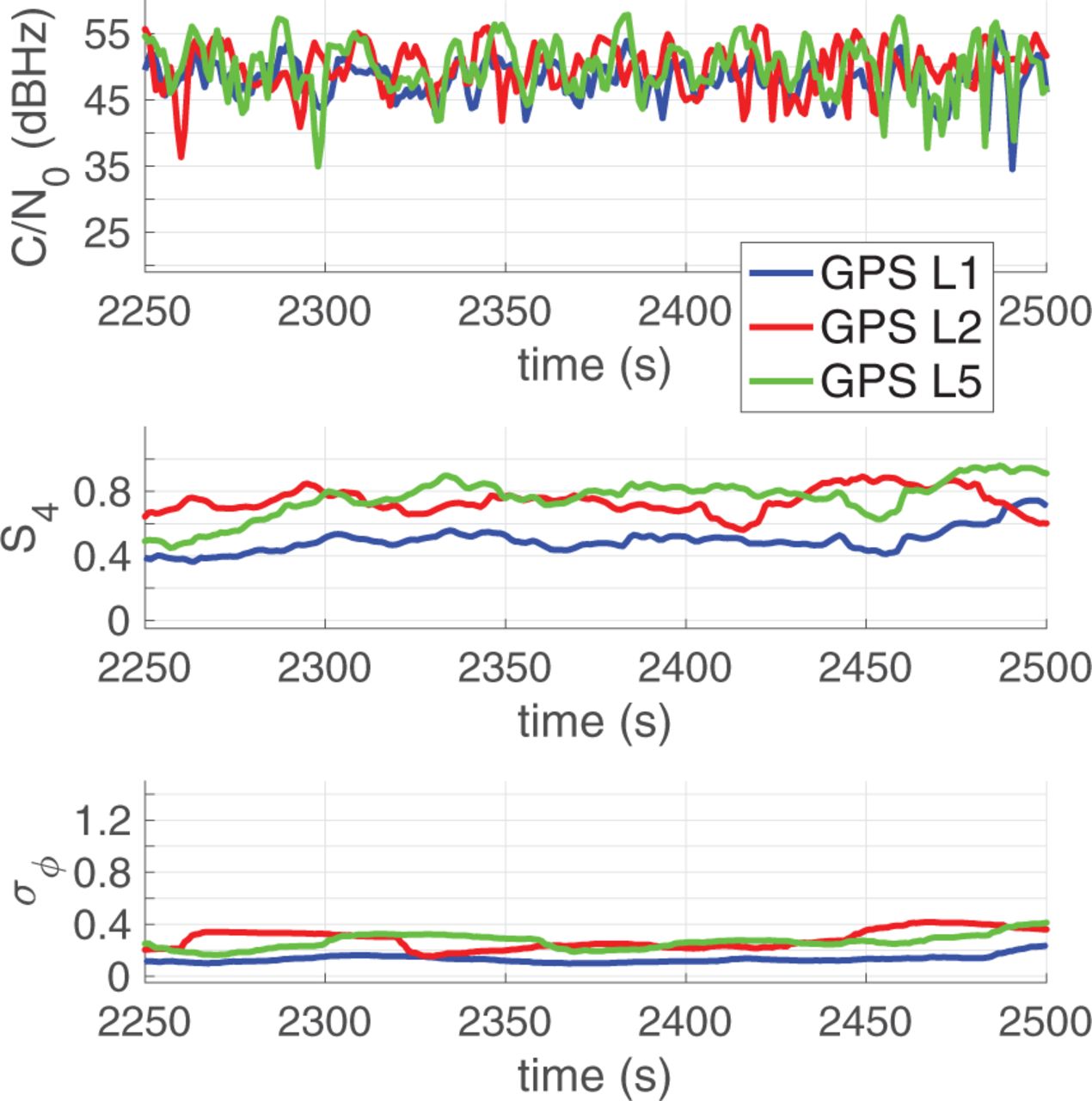
Moderate to strong (frequency dependent) equatorial amplitude ionospheric scintillation, with moderate phase scintillation. Event recorded over Hanoi, Vietnam, Spring 2015

• Download figure
• Open in new tab
• Download powerpoint

FIGURE 2

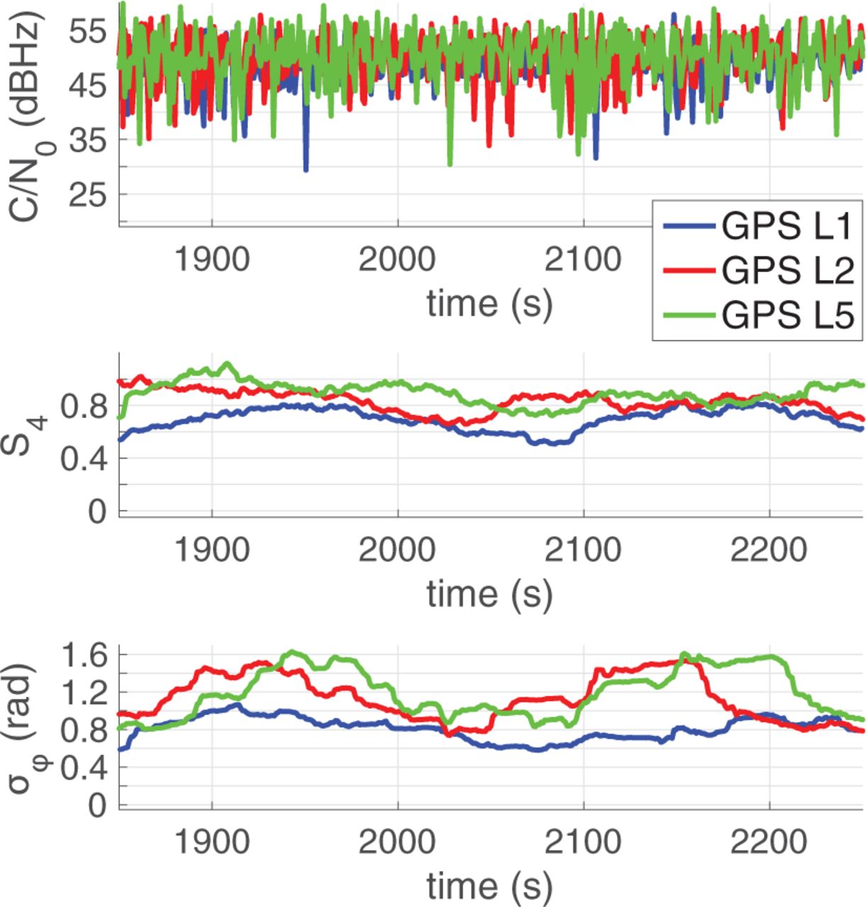
Severe equatorial amplitude and phase ionospheric scintillation. Event recorded over Hanoi, Vietnam, Spring 2015

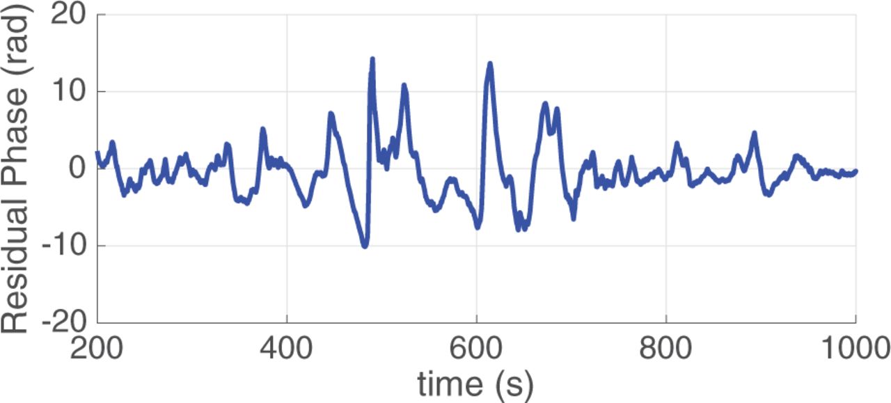
For the sake of completeness, Figure 3 shows a scintillation event at a high-latitude location (Svalbard Islands, Norway) recorded during September 2017. The recording involves single-frequency measurements, and the figure shows the indicators for two different satellites. Clearly, there is phase distortion appreciated around 400 − 600 seconds in the recording, as reported by the σ_φ estimate. Notice that in contrast with equatorial scintillation where both severe amplitude and phase variations may appear (i.e., high S₄ and σ_φ), high-latitude scintillation typically only affects phase variations, that is, there are no deep amplitude fades (i.e., low S₄).

• Download figure
• Open in new tab
• Download powerpoint

FIGURE 3

Single-frequency high-latitude ionospheric scintillation event recorded over Svalbard Islands, Norway, September 2017

3.1 Visual inspection

Most of the approaches in the literature, especially in the works where scintillation indices are used as input to advanced studies, are based on manual visual inspection of S₄ and σ_ϕ, as provided by professional commercial ISMR. Time series of scintillation indices spanning intervals of several hours and typically including all satellites in view from all constellations and frequencies available are observed, and the presence of scintillations is empirically evaluated. To help the classification, users often rely also on assistance from other measurements and instruments, such as CN0, TEC, ROT, satellites azimuth and elevation, Solar flare detectors, or magnetometers. Also, the comparison with historical data can help in some situations, due to the unique regularity pattern of scintillations. As an example, fluctuations of S₄ due to multipath can be easily recognized on GPS signals by examining the same time series at regular intervals of one sidereal day (Axelrad, Larson, & Jones, 2005). The rate of the observation is typically one minute, and the detection resolution is of the order of tens of minutes. Even though lacking of scientific rigor, this approach assures the best detection performance. The main drawbacks are that it is time consuming, not automatic and subject to errors dependent on knowledge and experience of the person performing the task.

3.2 Thresholding

More advanced and semi-automatized approaches are based on automatic event triggers, relying on the comparison of the value of the same scintillation indices with predefined thresholds. This approach is referred to as threshold trigger in Taylor et al. (2012) and as Hard detection rule in Linty et al. (2019), as it is a fully-automatized objective decision. Different thresholds can be defined for amplitude and phase scintillation, respectively, 𝒯_S4 and 𝒯_σϕ. A scintillation event is declared by the system when the indicator surpasses the threshold. When both S₄ and σ_ϕ are considered, then scintillation is declared present, at epoch n, if and only if:

10

The performance clearly depends on the choice of the threshold, which in turn depends on different and complex factors including location, time, environmental conditions, and quality of hardware and of oscillator. Overly conservative thresholds result in large missed detections rates, whereas overly aggressive thresholds lead to large false alarm rates. Concerning amplitude scintillation, 𝒯_S4 = 0.4 is chosen by many authors (Adewale et al., 2012; Aon, Othman, Ho, & Shaddad, 2015; Dubey, Wahi, Mingkhwan, & Gwal, 2005; Middlestead, 2017; Romero Gaviria, 2015); other works consider scintillation moderate in the range between 0.2 and 0.5 and strong above 0.5 (Jiao, Morton, Taylor, & Pelgrum, 2013a). Concerning phase scintillation, a common value is 𝒯_σϕ = 0.25 rad (Dubey et al., 2006; Linty, Minetto, Dovis, & Spogli, 2018). Sometimes, the same authors consider different thresholds depending on the type of study being carried out: 0.15 and 0.26 rad for amplitude and phase scintillation, respectively, to detect events potentially causing a considerable impact on GNSS measurement accuracy and reliability (Jiao, Morton, Taylor, & Pelgrum, 2013b), while 0.12 and 0.1 rad, for studies on the ionosphere irregularity (Jiao, Morton, Taylor, & Pelgrum, 2013a).

Both the rate of the observation and the detection resolution are equivalent to a one-minute observation interval. The advantages are the simplicity, the low computational burden, and the low tuning requirements. However, it is prone to undesired and non-negligible false alarms, due to ambiguity between real scintillations and other kinds of nuisances, especially in the case of amplitude scintillation.

In order to reduce false alarms and missed detections due to multipath and other propagation errors, and to better characterize the scintillation phenomenon, more sophisticated techniques have been proposed. For instance, when measurements other than σ_ϕ and S₄ are available, additional masks can be applied to the signal. It is quite common to apply an elevation mask; the majority of multipath-induced false alarms can be successfully removed by discarding signals below a certain elevation angle, at the expenses of the potential loss of relevant and useful information. A more advanced thresholding detection rule can be defined as follows: amplitude scintillation is present at epoch n if and only if:

11

where the value of the elevation threshold 𝒯_θel can be chosen depending on a priori evaluation of the surrounding area. A typical value is 30° (Abadi et al., 2014; Jiao, Morton, Taylor, & Pelgrum, 2013a).

Similarly, further conditions can be defined on the CN0, so as to exclude measurements which are too noisy; or on the satellites azimuth, to counteract specific environmental signals obstructions. However, the definition of the corresponding 𝒯_C/N0 is deemed more complex, as the CN0 strictly depends on the receiver implementation. The value 37 dB-Hz has been proposed as threshold in some studies (Linty, Dovis, & Alfonsi, 2018; Linty, Farasin, Favenza, & Dovis, 2019), while other authors propose to use 40 dB-Hz (Curran, Bavaro, Morrison, & Fortuny, 2015a), or even 30 dB-Hz, corresponding to the tracking-loop sensitivity (Van Dierendonck, 2009). Pelgrum et al. (2011) proposed an event trigger based on a joint S₄ and CN0 threshold, in the form:

12

where CN0 is in dB-Hz and 0.01875 is in units of (dB-Hz)⁻¹. According to Vikram et al. (2011), no false alarms were detected using this technique over a six-day data collection, at the expenses of a high missed detection rate (4 events detected out of 25), especially in the presence of phase scintillation.

An extension of this, taking into account also the σ_ϕ and satellites elevation was proposed in Vikram et al. (2011). To reduce the multipath effects, all entries below 30° were a priori eliminated. Scintillation is then declared present if one of the two conditions holds:

13

14

with θ_el expressed in degrees. This technique was further refined by adding a third condition on the satellites azimuth, based on empirical considerations on a set of data, and selecting the thresholds according to a user-specified false alarm rate and on a manual visual-based scintillation detection. A disadvantage of such an approach is that it relies on a minimization process on a certain distribution of data and does not scale well for different spatial and temporal observations. Furthermore, the same study of the authors reveals high false alarm rates. In general, despite a difference in the detection results that has been observed between summer and winter, this is negligible and a separate threshold setting for winter and summer is not necessary (Taylor et al., 2012).

In order to better filter data affected by multipath, more advanced masks can be defined. As multipath effects are location dependent, the environment surrounding the receiver can be characterized, to avoid losing valuable data by setting predetermined filtering masks. A location-specific azimuth-dependent elevation mask has been developed in Atilaw et al. (2017).

Another possible way to distinguish scintillation events from multipath is to rely on historical data and on the repeatability of GNSS satellites visibility. For instance, in the case of the GPS constellation, it is generally assumed that the GPS orbits repetition equals the sidereal day (23 hours, 56 minutes, and 4 seconds), although the precise amount of time shift may vary somewhat depending on the true satellite orbit (Axelrad et al., 2005). Therefore, also, multipath effects follow the same repeatability. The pattern induced by multipath on the S₄ can be considered deterministic and is observed with regularity, contrary to true scintillation events, which are inherently random. Spogli et al. (2014) proposed a method to filter out spurious data, including multipath affected signals, based on an “outliers analysis.” Such an approach can reduce the data loss from 35 − 45% to 10 − 20%.

3.3 Non-scintillation indices-based techniques

Approaches based on the sole analysis of the scintillation indices share a common drawback. S₄ and σ_ϕ, despite being widely recognized, overlook higher moment characteristics of the signals (Jiao, Hall, & Morton, 2017a). Their computation requires averaging and detrending operations and, in general, algorithms with complex tuning, which are time consuming, computationally expensive, and potentially introduce heavy artifacts, thus altering the scintillation detection process (Mushini et al., 2012). In particular, although detrending the phase by means of a Butterworth filter is the de facto standard (Van Dierendonck, Klobuchar, & Hua, 1993), many authors have shown limitations when dealing with polar scintillations, related to the choice of the filter cutoff frequency, which should be related to the local features of the ionosphere (Forte, 2005; Mushini et al., 2012; Ouassou et al., 2016). A wrong and non-adaptive cutoff frequency ultimately alters the value of the traditional indices up to the point in which the scintillation detection is completely mistaken. Furthermore, detection based on fixed thresholds can be misleading: a hard classification based on the definition of thresholds (no scintillation, moderate scintillation, strong scintillation) determines abrupt and sudden classification, often irrespective of the true physical process determining the event. Furthermore, transient phases of the events can be lost, causing a delay in the detection alert (Linty et al., 2019), while weak events with high variance can be missed. A fuzzy indication system giving a more reasonable expression of the scintillation depth has been proposed, to overcome the ambiguity existing in the numerical and linguistic definitions of scintillation intensity (Fu et al., 1999).

Alternatives to detection rules based on scintillation indices and thresholds usually exploit dedicated receiver architectures and possibly complex and computationally expensive operations. For these reasons real-time detection is usually not possible. One of the first techniques based on alternative analysis was proposed in Fu et al. (1999) and is based on wavelet decomposition. According to the authors, scintillation-related signal features can be effectively detected or extracted by transforming the time domain scintillation signals by means of orthonormal and compactly supported wavelet bases. Wavelet-based detrending has also been proposed in Mushini et al. (2012). Alternative scintillation indices, based on non-parametric local regression with bias Corrected Akaike Information Criteria (AICC) have been proposed by Ouasson et al., reducing the computational load of wavelet analysis and superior handling of discontinuities (Ouassou et al., 2016). Recently, the Adaptive Local Iterative Filtering (ALIF) method has been proposed to analyse phase time series, improving scale resolution with respect to wavelet transform (Piersanti et al., 2018).

When dealing with amplitude scintillation only, the analysis of CN0 allows detection of anomalous variations in the signal amplitude. In this case, it is even harder to distinguish between real scintillation and other impairments. However, the CN0 is a measure largely available in any GNSS receiver, including mass-market and non-professional devices, making CN0-based techniques cheap, accessible, and applicable also to historical data. In Miriyala, Koppireddi, and Chanamallu (2015), CN0 time series of GNSS data are decomposed exploiting adaptive time-frequency methods. In particular, the technique denoted complementary ensemble empirical mode decomposition showed good detection results.

More recently, and thanks to the widespread availability of raw IF samples of GNSS signals for scintillation monitoring (Cristodaro, Dovis, Linty, & Romero, 2018; Lachapelle & Broumandan, 2016), other approaches have been proposed, directly looking at lower processing stages of the receiver. The received signal samples contain information about scintillation, although buried in the noise floor. After removing the deterministic components of the signal (carrier frequency, modulating codes, and navigation message), and by filtering out noise exploiting averaging techniques, the contribution of scintillation can be isolated. An open-loop approach was proposed in Romero et al. (2016) and Linty and Dovis (2019); a metric alternative to the S₄ was suggested to detect amplitude scintillation, based on the evaluation of the statistical properties of the histogram of the received samples. Different techniques were evaluated, such as skewness and goodness of fit, obtaining high detection, low false alarm, and low missed detection rates when compared to the S₄-based thresholding. Despite requiring a dedicated receiver architecture, this approach is insensitive to the degradation of the results due to strong scintillations, which might impact on the receiver tracking loops and thus falsify the traditional detection.

3.4 Machine learning

Recent studies have proposed machine learning techniques for automatically detecting scintillation events. A machine learning process refers to the ability of solving a task by processing right features describing the domain of interest, according to a model built upon training on a set of historical data, which in the case of supervised learning are pre-labelled by manual annotation. More details about machine learning can be found in general purpose books, such as Flach (2012).

The selection of the set of features to be used in the training and in the classification tasks is the key aspect of machine learning algorithms. A clear strategy envisages the use of high-level observables, including the amplitude- and phase-scintillation indices, the signal CN0, and the satellites’ elevation and azimuth. This was first done exploiting SVM for the detection of amplitude scintillation in Jiao, Hall, and Morton (2016) and Jiao, Hall, and Morton (2017a). The algorithm was trained using a large amount of real scintillation data, manually labelled, and showed detection accuracy in the range 91-96%, outperforming other triggering systems analyzed. Some benefits were observed by including a further feature, corresponding to the Fourier Transform of the S₄ time series along an observation period of three minutes. A similar approach, targeting phase scintillation, was presented in Jiao, Hall, and Morton (2017b) and Jiao, Hall, and Morton (2017c), leading to detection accuracy around 92%.

Other works propose to use decision tree algorithms and low-level signal observables, such as the in-phase and quadrature correlation outputs of the receiver tracking loop (Favenza et al., 2017; Linty et al., 2019). The authors proved that the amplitude-scintillation detection accuracy is as good as 96.7% when S₄, CN0, and satellite elevation are used as features, but increases to 98.0% when using only correlator outputs and their combinations. Results further improve (99.7%) when using random forest algorithms at the expense of large computational loads. The authors also show how this approach is able to reduce the rate of false alarms due to the ambiguity between scintillation and multipath typical of the approaches based on the analysis of the S₄. Decision tree algorithms are also able to detect the transient time before and after the strongest phase of an event, thus providing an early run-time alert. Another advantage is that by exploiting the high-rate correlator outputs, a finer time resolution in detection is obtained. Furthermore, avoiding the use of the scintillation indices prevents any issue with the detrending and filtering processes. It is also important to mention that while the training phase to build the model can be computationally demanding, the decision phase is typically simple enough to be done in real time and with no impact on performance.

More recently, semi-supervised scintillation detection based on DeepInfomax technique has been proposed (Franzese, Linty, & Dovis, 2020). The method shows a classification accuracy in line with Linty et al. (2019), while reducing the amount of time required to manually label the training dataset, thus overcoming the drawbacks of supervised algorithms and advancing towards realistic deployment of machine learning-based scintillation detection. More generally, in Rezende et al. (2010), the authors propose a survey of data mining techniques for the prediction of ionospheric scintillations, relying on the observation and integration of GNSS receivers, other sensors, and online forecast services. This approach relies on external data sources and instruments.

5.1 Single-frequency synchronization

Traditional single-frequency synchronization (i.e., considering each satellite to receiver link independently) relies on well-known closed-loop DLL/PLL architectures (Kaplan, 2006) (see Section 2). When dealing with scintillation mitigation, state-of-the-art solutions attempt to render these classical approaches more robust, typically using heuristic adjustments (López-Salcedo, Peral-Rosado, & Seco-Granados, 2014; Yu et al., 2006). For instance, Skone et al. (2005) proposed an adaptive bandwidth PLL, which was coupled to a prediction model in Tiwari, Skone, Tiwari and Strangeways (2011). Other approaches rely on the combination of FLLs with PLLs (Fantinato, Rovelli, & Crosta, 2012; Mao, Morton, Zhang, & Kou, 2010; Zhang & Morton, 2009), extending the coherent integration time (Kassabian & Morton, 2014) and coupling with inertial sensors or Doppler-aided solutions (Chiou, 2010; Chiou, Gebre-Egziaber, Walter, & Enge, 2007; Chiou, Seo, Walter, & Enge, 2008). These techniques are somehow designed to avoid the loss-of-lock, with the main goal being to maintain a correct DLL tracking under scintillation conditions, which is only useful in standard code-based receivers. But, the limitations of standard locked-loop architectures are inherited by all these methods (Vilà-Valls, Closas, Navarro, & Fernández-Prades, 2017).

Some contributions have recently shown that an optimal filtering approach based on Kalman filtering (KF) (Anderson & Moore, 1979) provides better performance and robustness to scintillation (Barreau, Vigneau, Macabiau, & Deambrogio 2012; Humphreys, Psiaki, & Kintner, 2005; Macabiau et al., 2012; Zhang, Morton, Van Graas, & Beach, 2010), being nowadays the performance benchmark for the development of new methodologies. To avoid the complexity of the optimal Kalman gain computation (which is obtained from the prediction and estimation noise covariances, together with the system noise covariance matrices), these typically consider a constant gain KF implementation and then lose the optimality of the filter. Because the actual receiver working conditions are unknown to some extent, solutions based on adaptive KF (AKFs) have been studied in Zhang, Morton, and Miller (2010); Won, Eissfeller, Pany, and Winkel (2012); Won (2014); Susi, Aquino, Romero, Dovis, and Andreotti (2014); Susi, Andreotti, and Aquino (2014); and Xu, Morton, Jiao, and Rino (2017), which aim at sequentially adapting the filter parameters. Notice that the correct estimation of both noise covariance matrices is not possible due to identifiability issues (Vilà-Valls, Closas, & Fernández-Prades, 2015a), then typically only the measurement noise is adjusted. Some of the standard noise estimation techniques based on covariance matching and the autocorrelation of the innovation function (Duník, Straka, Kost, & Havlík, 2017) were evaluated in Vilà-Valls, Fernández-Prades, Closas, and Arribas (2017) and a new approach based on Bayesian covariance estimation in LaMountain, Vilà-Valls, and Closas (2018); the latter being a very promising approach.

From a signal-processing perspective, all the PLL/KF-based solutions above claim robustness against ionospheric scintillation, but this is done only by ensuring a certain robustness against cycle slips and loss-of-lock (i.e., increasing the noise uncertainty under scintillation conditions, so that the KF relies more on the LOS phase prediction model than on the current observation). But such an approach does not provide an effective mitigation of the harsh propagation conditions of interest. The question is how to design a method which minimizes the LOS carrier-phase estimation error. This leads to the estimation versus mitigation (EvM) dichotomy (Vilà-Valls et al., 2015a), which implies that a filter tracking the complete signal phase is not able to decouple the phase contribution due to the receiver dynamics of interest from the phase changes due to scintillation. A new approach to overcome these limitations was first proposed in Vilà-Valls et al. (2013) and later extended in Vilà-Valls, Closas, and Fernández-Prades (2015b) and Vilà-Valls et al. (2015a, 2018), where the scintillation physical phenomena is mathematically modeled as an autoregressive (AR) process, and embedded into the state-space formulation, which allows decoupling both phase contributions of interest. This method has been tested using both synthetic and real data, providing very promising performance results. Recently, to increase robustness in time-varying scenarios, adaptive AR parameter estimation techniques have been considered in Vilà-Valls, Fernández-Prades, Closas, and Arribas (2017) and Fohlmeister et al. (2018), showing that the approach in Vilà-Valls, Closas, Fernández-Prades, and Curran (2018) is the latest trend on single-frequency scintillation mitigation, and must be seen as the performance benchmark for the derivation of new scintillation mitigation strategies.

5.2 Multi-frequency synchronization

It is known that the ionospheric scintillation effects are frequency and latitude dependent (see Section 2). For instance, while in equatorial regions, a receiver experiences severe amplitude scintillation, and in high latitudes, the phase scintillation is the dominant part. Multi-frequency receivers (i.e., using GPS L1 C/A, L2 and L5) try to exploit the different scintillation characteristics at different frequency bands, with the aim to exploit the fact that not all the frequencies are equally degraded at the same time. As an example, deep amplitude fades in equatorial scintillation have low correlation (Seo, 2010), the reason why multi-frequency processing increases the robustness to scintillation (Carroll et al. 2014; Najmafshar, Ghafoori, & Skone, 2013; Psiaki, Humphreys, Cerruti, Powell, & Kintner, 2007; Seo & Walter, 2014). As stated for the single-frequency case, relying on standard multi-frequency PLL/KF-based architectures is not a good approach from a signal-processing perspective, because the filters track the complete phase of the signals, losing the capacity to effectively isolate the LOS and scintillation phase contributions.

The AR-based scintillation modeling within a KF-like architecture in Vilà-Valls, Closas, Fernández-Prades, and Curran (2018) was extended to the multi-frequency case in Vilà-Valls, Closas, and Curran (2017b) and Vilà-Valls, Closas, and Curran (2017a), using a multi-frequency state-space model formulation and a multivariate AR scintillation model. It was shown that exploiting both multi-frequency measurements and the scintillation approximation embedded into the filter improves the overall performance and robustness.

5.3 Multi-frequency/Multi-satellite solutions

There has been substantial research on combined multi-frequency/multi-satellite receivers to counteract scintillation (Lin, Lachapelle, & Souto Fortes, 2014). The easiest way to cope with such disturbance is to properly modify the navigation solution, typically weighting the pseudorange observables affected by scintillation (Aquino et al., 2007; Strangeways & Tiwari, 2013; Warnant et al., 2009), but from a signal-processing perspective, more sophisticated approaches can be considered. At the position level, another possible solution is to switch between phase and pseudorange observables when an event is detected (Myer et al., 2017).

In order to address some of the limitations of standard scalar synchronization techniques, mainly for weak signal environments and high-dynamics scenarios, several vector synchronization architectures (VTL) have been proposed in the last two decades (Giger, Henkel, & Günther 2009; Henkel, Giger, & Gunther, 2009; Lashley, Bevly, & Hung, 2009; Marçal & Nunes, 2016; Spilker, 1996). These solutions take advantage of the joint multi-channel (vector) processing, then making possible the meaningful exchange of information between channels. The goal is that channels under benign nominal conditions help the channels, which are corrupted by harsh propagation conditions, lowering the tracking threshold and thus increasing the satellite availability. These vector architectures have been shown to provide better position accuracy and increased robustness under non-nominal conditions w.r.t. standard scalar architectures. It is not the goal of this article to describe in detail the different vector-tracking architectures (i.e., vector DLL, vector DFLL, vector PLL, differential VPLL, partitioned vector tracking, etc.). Refer to the references provided and references therein for a deeper insight on pros and cons of the different approaches available in the literature.

These vector-tracking techniques have also been recently evaluated under ionospheric scintillation propagation conditions (Deambrogio & Macabiau, 2013; Marçal, Nunes, & Sousa, 2016, 2017; Peng, 2012; Sousa & Nunes, 2014a, 2014b; Xu, Jade Morton, Jiao, Rino, and Yang, 2018) in order to robustify the overall navigation solution. Even if the performance degradation of vector architectures under ionospheric scintillation is smaller when compared to standard (DLL/PLL) scalar-tracking techniques, including scintillation-affected satellites into the vector solution is not a good option. Using scintillation detection techniques to discard those satellites affected by scintillation from the navigation solution seems to be a better option, but this is not possible in situations with low satellite visibility. Then, from a signal-processing perspective, vector synchronization strategies may not be a good approach, at least in their current status. Notice that the advanced signal-processing techniques described in Sections 5.1 and in 5.2 can also be used in multi-frequency/multi-satellite configurations to improve the overall system performance, taking the best of both worlds.

6.1 Examples of scintillation detection

An overview of scintillation detection results is provided in this section. The techniques described in Section 3 are applied on the example datasets presented in Figures 2 and 3. Only qualitative results are shown, as a complete statistical analysis on detection techniques would require to consider a much larger input dataset, representative of any possible physical and environmental conditions. Moreover, each of the techniques presented targets a specific monitoring need, thus it is not possible to compare them in a unified way. For these reasons, the figures shall be considered illustrative and not conclusive; the readers interested can delve into the appropriate references provided.

Figure 4 reports a time series of S₄, CN0 and elevation of GPS PRN 30 on April 2, 2015 at equatorial latitudes. The yellow boxes throughout the S₄ trace identify the portions of data affected by amplitude scintillation, according to a manual visual inspection of the dataset. Even though after minute 15:22 the elevation is lower than 30°, the analysis of historical data and of the station environment assures that multipath cannot be held responsible for such an increase of the amplitude-scintillation index. The detection results are depicted in the top panel of the figure. The simple thresholding rule of Equation (10) marks as scintillation all the points for which S₄ is larger than 𝒯_S4 = 0.4. Carefully analyzing, it appears that the rule fails in detecting the exact start and end of each event. When the mask on the elevation is also applied, as defined in Equation (11), all points after minute 15:22 are discarded, resulting in a large missed detection rate. The detection rule of Equation (12) shows very good results, well aligned with the event visual inspection. On the contrary, the results of Equation (13) mark as scintillation all the points of the time series. This is probably due to the high noise floor of the S₄ estimate, potentially due to the bad quality of hardware used for the data collection. A slight modification of the equation would be required, performing a calibration on data not affected by scintillation. The green line reports the detection results of a decision tree machine learning technique using as observables the correlator outputs, as proposed in Linty et al. (2019). The training phase was performed on other data captured at the same station during different events.

• Download figure
• Open in new tab
• Download powerpoint

FIGURE 4

Example of amplitude detection results on data captured on April 30, 2015, GPS PRN 30, L1 C/A

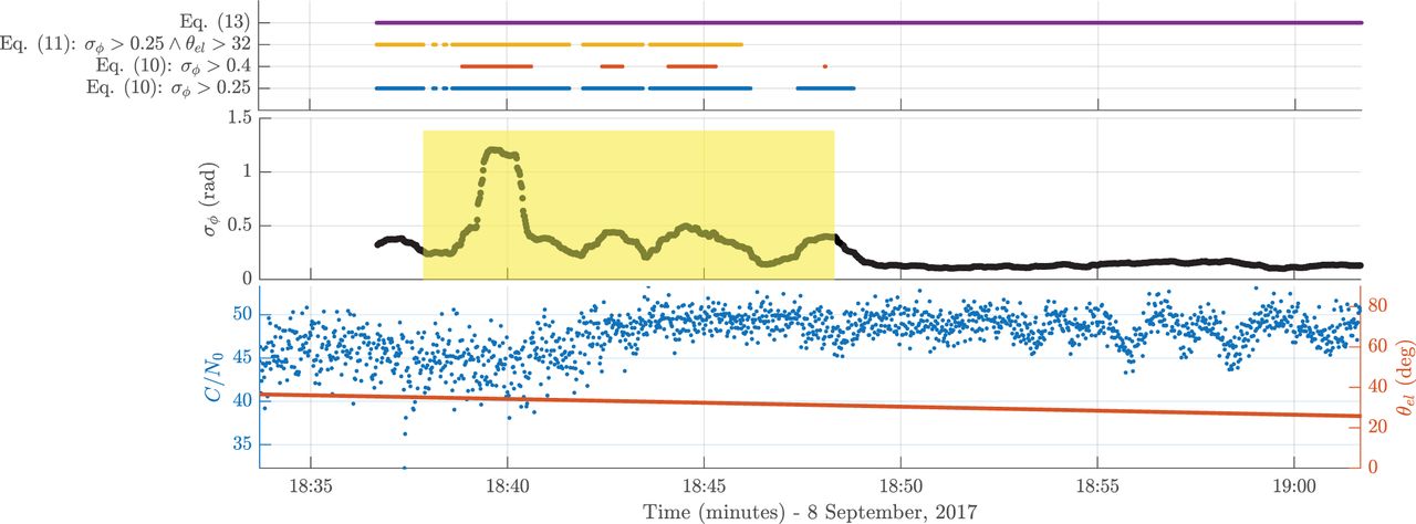
Similarly, qualitative results of the phase-scintillation detection methods are reported in Figure 5. σ_ϕ, CN0 and elevation times series of GPS PRN 6, on September 8, 2017, at high latitudes, are reported. As above, the yellow box marks the start and end of the phase-scintillation event, according to visual inspection. The hard rule of Equation (10) is reported for two different thresholds, 𝒯_σϕ = 0.25 rad and 𝒯_σϕ = 0.4 rad. In the first case, the detection result almost matches the performance of the manual inspection, but misses a few points, which despite showing a σ_ϕ lower than the threshold are clearly part of the same scintillation event. Adding also the elevation mask, according to Equation (11), brings no benefits; however, this is due to the fact that no multipath is present in this specific data acquisition. The rule defined in Equation (13) is also reported, but as in the case of amplitude scintillation, it fails due to the high noise floor of the σ_ϕ estimation. Also, in this case, a calibration phase would be required.

• Download figure
• Open in new tab
• Download powerpoint

FIGURE 5

Example of phase detection results on data captured on September 8, 2017, GPS PRN 6, L1 C/A

It is clearly not possible to identify the optimum technique, according to detection results of a single event, and with no specification about the target application. High-end receivers have different requirements, in terms of scintillation detection, compared to mass-market receivers and to receivers for space weather monitoring. Similarly, certain applications require the detection of events which are harmful for the capability of the GNSS receiver to produce a correct position estimate; other applications require the detection of events significant under a physical point of view. In general, improved processing capabilities allow nowadays the design and implementation of very advanced detection schemes, reaching very high detection rates and low false alarms.

6.2 Example of high-latitude scintillation monitoring

As already stated, ionospheric scintillation monitoring is of paramount importance for several scientific applications (Coster, Gaposchkin, & Thornton, 1992; Doherty, Coster, & Murtagh, 2004; Goncharenko, Chau, Liu, & Coster, 2010; Goncharenko, Coster, Chau, & Valladares, 2010). The main limiting factor for the use of low-cost mass-market GNSS receivers for this purpose (i.e., to avoid high-cost professional dedicated ISMR with very stable clocks and perfectly known position) is the clock-induced phase errors. Considering the architecture proposed in Vilà-Valls, Closas, and Curran (2017a), we show new results for a high-latitude scintillation event, recorded in September 2017 over Longyearbyen, at the Svalbard Islands, Norway (Linty, Minetto, Dovis, & Spogli, 2018), using a customized receiver developed by the NavSAS group of Politecnico di Torino (Cristodaro et al., 2018). As a low-cost receiver clock example, we consider a typical temperature-compensated crystal oscillator (TCXO), for which we measured the clock-phase-induced errors. The characterization of the scintillation event is shown in Figure 3 (PRN 9) where there is no amplitude scintillation but phase scintillation is clearly present, as expected for a high-latitude ionospheric scintillation event. In this exemplary case, the phase residual to be tracked is shown in Figure 6. Recall that this phase residual is the output of the DLL prompt correlator, then it depends on the integration time, i.e., T_I = 10 ms in this case. Notice that this integration time is purposely chosen to show a challenging scenario, for instance compared to a T_I = 1 ms choice, which would induce slower phase variations and thus be easier to track at the receiver.

• Download figure
• Open in new tab
• Download powerpoint

FIGURE 6

Real ionospheric scintillation event recorded over Svalbard Islands, Norway, September 2017. The scintillation-induced phase variations to be estimated are shown for T_I = 10 ms

At the receiver, we consider a nominal C/N₀ = 40 dB-Hz and a coherent integration time of T_I = 10 ms. The root-mean-square error (RMSE) for the estimation of the TCXO clock-induced phase variations (i.e., computed from a scintillation-free satellite link) is 0.0574 radians. This estimated clock phase is used to compensate the clock error in the scintillation affected satellite link. In Table 3, we show the monitoring capabilities of the AR-based KF. The different values correspond, left to right, to the RMSE for the estimation of the scintillation phase variations without any clock-phase error, the RMSE for the estimation considering a compensated clock from the scintillation-free satellite link, and the RMSE for the estimation without compensating the clock-phase errors. It is clear that a bad quality clock has a huge impact on the receiver, not being able to correctly estimate the scintillation phase of interest because the filter tracks the complete phase (scint + clock). But correctly using a clock estimation procedure provides a good scintillation phase estimate, which opens the door for low-cost monitoring architectures, boosting new scientific applications.

6.3 Example of adaptive multi-frequency severe equatorial scintillation mitigation

To close the loop and give a better insight on the synchronization performance, we show new results for a robust scintillation mitigation example. We assess the performance of different methods using real equatorial data recorded during high ionospheric activity. The real triple-frequency (L1, L2 and L5) amplitude- and phase-scintillation time series are obtained from the Joint Research Centre (JRC) Scintillation Repository, recorded over Hanoi in March and April 2015. To obtain the clean ionospheric scintillation time series, a multi-frequency open-loop software receiver was used for post-processing the original datasets (Curran, Bavaro, Morrison, & Fortuny, 2015a, Curran, Bavaro, Morrison, & Fortuny, 2015b). We propose a new adaptive multi-frequency architecture, where the approach originally derived in Vilà-Valls, Closas, and Curran (2017a) is combined with a sequential multivariate AR parameters estimation method (named MF-On-ARKF). This method is compared to:

• i. A third-order fixed bandwidth (B_w = 15 Hz) PLL.

• ii. An AKF, adjusting the phase noise variance at the discriminator output from the estimated CN0.

• iii. A single-frequency AR-based KF sequentially estimating the AR parameters (SF-On-ARKF) (Vilà-Valls, Fernández-Prades, Arribas, Curran, & Closas, 2018).

• iv. A single-frequency AR-based KF with off-line fitting to the real scintillation data (SF-Off-ARKF) (Vilà-Valls, Closas, Fernández-Prades, & Curran, 2018).

• v. A multi-frequency AR-based KF with off-line fitting to the real scintillation data (MF-Off-ARKF) (Vilà-Valls, Closas, & Curran, 2017a).

Notice that both SF-Off-ARKF and MF-Off-ARKF are the performance benchmarks for single and multi-frequency processing. We show the characterization of the severe scintillation event under study in Figure 7, where it is clear that there is both amplitude and phase scintillation. From the second zoom plot in Figure 7, we can see that the deep fades at different frequency bands are uncorrelated, a fact that can be exploited using multi-frequency architectures. We consider an initial Doppler f_d,0 = 50 Hz and rate f_r,0 = 10 Hz/s, a nominal C/N₀ = 40 dB-Hz, and coherent integration T_I = 10 ms. The measure of performance is the RMSE on the carrier phase of interest at L1 and the RMSE for both scintillation components for the methods based on the AR approximation. The RMSE results are given in Table 4. We can see that including the AR scintillation modeling into the state-space formulation, then being able to decouple both phase contributions, drastically improves the mitigation capabilities. Moreover, multi-frequency processing further improves the estimation results. The performance improvement is even more obvious considering L2 and L5 signals, where the scintillation effects are always more severe (Vilà-Valls, Closas, & Curran, 2017a).

• Download figure
• Open in new tab
• Download powerpoint

FIGURE 7

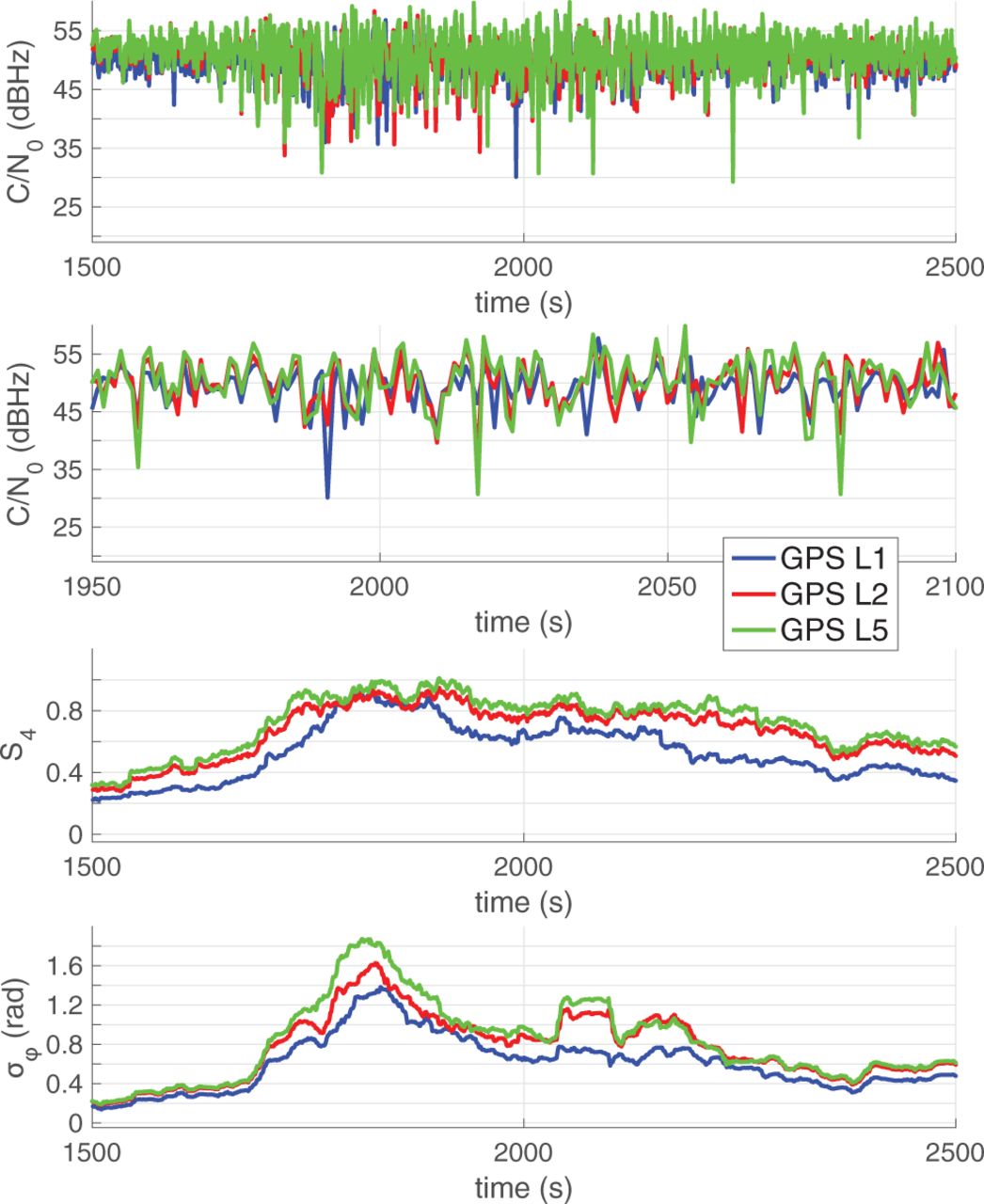
Real equatorial ionospheric severe scintillation event recorded over Hanoi, Vietnam, Spring 2015. The two top plots show the C/N₀ for the whole sequence and a zoom to clearly see that deep fades at different frequency bands are uncorrelated