

Abstract
In this paper, we propose a machine-learning-based approach to automatically detect a satellite oscillator anomaly. A major challenge is to differentiate an oscillator anomaly from ionospheric scintillation. Although both scintillation and oscillator anomalies cause phase disturbances, their underlying physics are different and, therefore, show different carrier-frequency dependency. By using triple-frequency signals, distinct features are extracted from the disturbed signals and applied to the radial basis function (RBF) support vector machine (SVM) classifier to identify an oscillator anomaly. The results show that the proposed RBF SVM displays superior performance and outperforms several other classification methods. The proposed approach is applied to an extensive GNSS database to conduct automatic satellite oscillator anomaly detection. Preliminary detection results validate the effectiveness of the proposed method. On average, one-to-three satellite oscillator anomaly events are detected daily at each receiver location.
- global monitoring system
- kernel trick
- machine learning
- phase scintillation
- satellite oscillator anomaly
- support vector machine
1 INTRODUCTION
Global navigation satellite systems (GNSS) have been playing an essential role in everyday life, and reliable signal quality is the foundation of many critical applications (Fernholz, 2018). Thus, signal-quality monitoring is an important task to provide timely correction and warning to GNSS users (U.S. Department of Defense, 1993). Various aspects of the signal, including signal power, cross correlation, carrier-phase anomaly, excessive acceleration, signal deformation, etc. (Houston, Liu, & Brenner, 2001; Navigation Systems Panel [NSP], 2016; RTCA DO-253D, 2017; US DOT, 2009), need to be monitored to ensure a guaranteed level of performance. Among the various signal parameters, carrier-phase anomaly could lead to service discontinuity, loss of correction service coverage, or even service outage, especially for high-accuracy/integrity applications (Vary, 2012). A satellite oscillator anomaly is one of the causes of carrier-phase disturbances and affects all users that rely on its signal integrity (Weiss, Shome, & Beard, 2006). Therefore, it is important to monitor it and broadcast warnings of the potential anomalies.
A satellite oscillator anomaly has been observed in several past studies (e.g., Benton & Mitchell, 2012, 2014). In Benton and Mitchell (2012), a GPS L1 signal from PRN 13 was observed to have pulses of rapid phase variations caused by a satellite oscillator anomaly. In Benton and Mitchell (2014), satellite oscillator anomaly events were observed from a modern block IIF satellite (PRN 1). However, these satellite oscillator anomaly events were observed by visual inspections of carrier-phase measurements. This is obviously impractical for a global satellite oscillator anomaly monitoring system. Furthermore, an oscillator anomaly usually needs to be alerted in a timely manner for the most stringent requirements of safety-critical services, such as aircraft navigation (Vioarsson, Pullen, Green, & Enge, 2001; Weiss, Shome, & Beard, 2010). Ground-based satellite operator solutions to this problem have difficulty alerting users of the anomaly in a timely manner. Thus, automatic detection is desired.
In Heo, Cho, and Heo (2012), the authors proposed to use the Teager Energy operator to detect sudden changes caused by oscillator anomalies. The method assumes that the ionospheric effect can be removed by either using dual-frequency measurements or the Klobuchar model. However, these assumptions are not valid. The ionosphere-free dual-frequency combination can only remove the first-order ionospheric refraction effect (McCaffrey & Jayachandran, 2017). Ionospheric scintillation is typically due to a combination of refraction and scattering or diffraction of the signal propagating through plasma structures. The diffractive contribution introduces additional disturbance and cannot be removed by the dual-frequency measurements or ionospheric models (Carrano, Groves, McNeil, & Doherty, 2013; McCaffrey & Jayachandran, 2019; Morton et al., 2020). Therefore, this approach will not be effective. Even in the absence of ionospheric scintillation, the dual-frequency differencing approach cannot distinguish satellite oscillator anomalies from receiver oscillator anomalies. To address these issues, the authors in (Ramesh, Ugazio, & van Graas, 2017) proposed using two nearby receivers to detect the satellite oscillator anomaly. The distance between the two receivers should be close enough to have a common view of the same satellite in the sky, but far enough to ensure that environmental errors are decorrelated. A satellite oscillator anomaly is then identified when both receivers observe the same anomaly. A major shortcoming of this approach is that the requirement of two receivers makes it difficult to be deployed on existing monitoring systems and any updates to this existing system will be costly.
In this paper, we propose a machine-learning-based approach to detect satellite oscillator anomalies using triple-frequency measurements from a single receiver. It involves a three-step process. First, phase disturbance events are detected by using the linear support vector machine (SVM)-based machine-learning algorithm presented in Jiao, Hall, and Morton (2017). The triple-frequency carrier-phase measurement segments are identified based on the linear SVM detection outputs. Then, features are extracted from triple-frequency signals and applied to a radial basis function (RBF) SVM to distinguish between ionospheric scintillation and oscillator anomaly. Finally, the anomaly will be classified as a receiver oscillator anomaly if the detected oscillator anomaly is presented on measurements from multiple satellites in view. Otherwise, it is classified as a satellite oscillator anomaly.
The rest of the paper is organized as follows: Section 2 introduces the linear and RBF SVM-based machine-learning concepts, followed by the proposed satellite oscillator anomaly detection approach in Section 3. Section 4 evaluates the performance of oscillator anomaly detection. Preliminary detection results are presented in Section 5. Finally, concluding remarks and future work are presented in Section 6. Note that we use the terms scintillation and phase scintillation interchangeably in this paper, where both terms refer to carrier-phase scintillation.
2 SUPPORT VECTOR MACHINE
SVM is a supervised learning algorithm that deals with classification problems (Bishop, 2006; Cortes & Vapnik, 1995; Jiao et al., 2017). It is known to be one of the best algorithms for solving classification tasks that are not linearly separable. Suppose that we have a training dataset with m samples D = {(x(1), y(1)), (x(2), y(2)), …, (x(m), y(m))}, where x(i) ∈ ℝn, i = 1,…, m denotes the feature vector and y(i) ∈ ℝ, i = 1, …, m is the corresponding label. The primal form of the SVM objective function is
 1
1
where ω ∈ ℝn and b ∈ ℝ are the weight and bias, respectively. ξi ∈ ℝ, i = 1,…,m are the slack variables for each sample in the training dataset, and C is a hyperparameter that determines the importance of the second term in the objective function. The hyperparameter’s value is set before the training process begins. Usually the optimal hyperparameter can be obtained by cross-validation (Bishop, 2006). In general, the objective of training an SVM classifier is to find a hyperplane that maximizes the distances to the nearest sample points on each label (first term in Equation (1)) and minimizes the misclassified samples’ distances (second term in Equation (1)) (Bishop, 2006). By solving this objective function, the optimal variables ω∗, b∗,  , i = 1,…,m can be obtained. To make a decision on an unseen sample with features x′, we can run the decision function
 2
2
A positive label is assigned when  and vice versa.
The decision function in Equation (2) is linear and, thus, may behave poorly if the problem is not linearly separable. To overcome this, the convex property of SVM is utilized to transform the primal form of the objective function (Equation (1)) to an equivalent dual form:
 3
3
where ⟨⋅, ⋅⟩ is the inner product and α ∈ ℝm.
As a property of convexity, the primal form and dual form are equivalent and the solution of one form can be derived from the solution of the other (Boyd & Vandenberghe, 2004). As a result, we could find the decision function via Equation (3) rather than Equation (1). This gives us an equivalent decision function as
 4
4
where the bias b can be derived from α (details can be found in Bishop, 2006). This decision function is equivalent to Equation (2) as the Karush-Kuhn-Tucker condition (Boyd & Vandenberghe, 2004) shows that  With this equivalent decision function, a kernel trick can be played on this dual form by replacing the inner product with a kernel operation:
 5
5
where φ(⋅) is a feature mapping function. For instance, the original decision function uses a linear feature mapping function φ(x) = x.
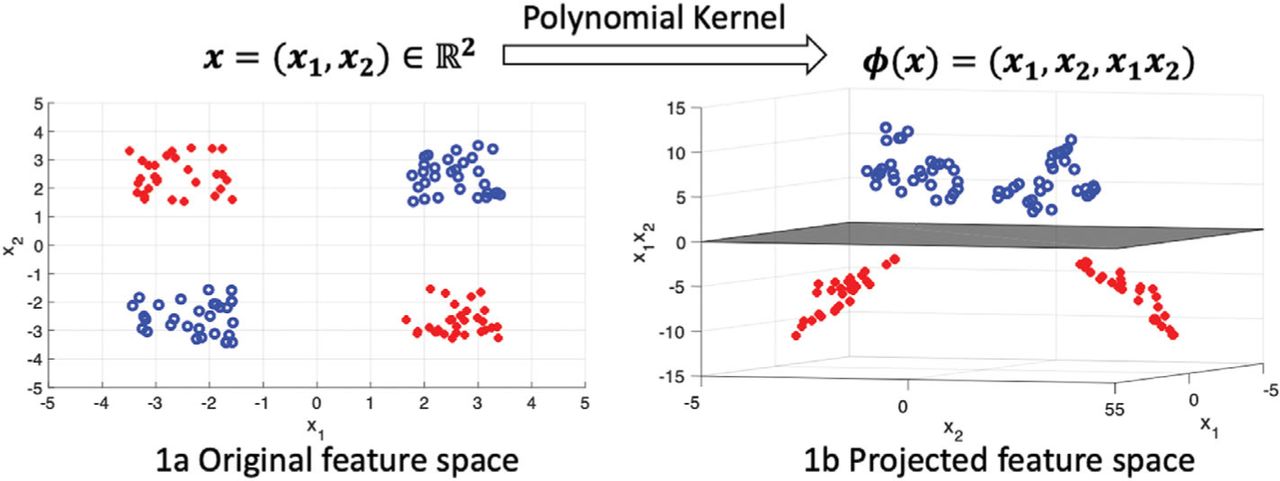
The introduction of the kernel trick in the inner product maps the original features onto a higher dimensional feature space. This mapping could potentially transform a non-linearly separable problem to a linearly separable problem. Let us assume that we have a non-linearly separable problem in a 2D feature space as shown in Figure 1a. Each dot/circle represents a data sample, and the color of the sample represents its label. In the feature space, each sample is represented by a feature vector x = (x1,x2) ∈ ℝ2. It is clear that this is a non-linearly separable problem because it’s impossible to find a straight line to separate these two classes. A polynomial kernel can be applied by using a feature mapping function φ (x) = (x1,x2,x1x2) to map each sample to a 3D space as shown in Figure 1b. In this 3D feature space, the problem is linearly separable, shown by the gray hyperplane.

An illustration of the kernel trick. The data is not linearly separable in the original 2D feature space (left), but is linearly separable in the mapped 3D space (right)
In practice, it is not straightforward to design an optimal polynomial kernel for a specific task. To tackle the non-linearly separable problem, a commonly used kernel is the RBF kernel:
 6
6
where γ is a hyperparameter and ‖⋅‖ is the Euclidean norm. In theory, this kernel maps the original feature space with limited dimensions to a feature space with infinite dimensions. This gives the SVM the ability to classify samples in an infinite dimensional feature space, which offers better separation between classes. Therefore, an RBF kernel could be applied to improve the classification performance. In a subsequent section, we will show that oscillator anomaly detection is a non-linearly separable problem. Hence, the RBF kernel can be applied.
3 SATELLITE OSCILLATOR ANOMALY DETECTION
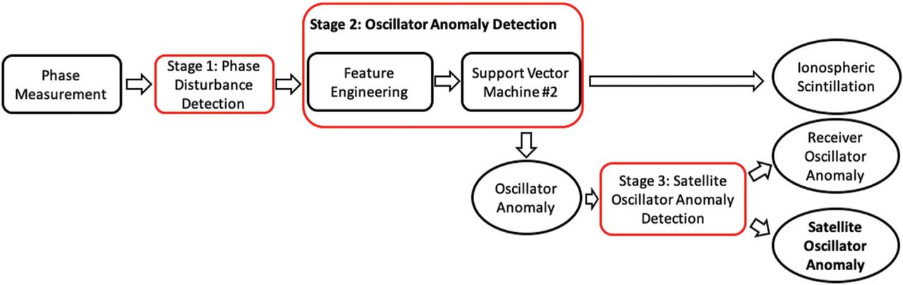
To identify a satellite oscillator anomaly event, three stages are involved. First, a linear SVM (SVM #1) is implemented to detect phase disturbances. Second, an RFB SVM (SVM #2) is applied to the detected phase disturbances to identify an oscillator anomaly. Finally, the differentiation between satellite oscillator anomaly and receiver oscillator anomaly is conducted. A block diagram is shown in Figure 2 to illustrate the process.

Satellite oscillator anomaly detection block diagram
3.1 Stage 1: Phase disturbance detection
This first stage aims to identify phase disturbance events in phase measurements. To do so, the SVM #1 using frequency domain features of the L1 signal is employed. Readers are referred to Jiao et al. (2017) for a thorough description and performance analysis of the phase disturbance detection. Note that the phase measurement data is divided into three-minute windows to ensure there are sufficient samples to capture the phase oscillation. Therefore, each detected phase disturbance event is also three minutes long. Subsequent visual inspections will identify the actual disturbance duration from the collection of three-minute long events.
3.2 Stage 2: Oscillator anomaly detection
As both oscillator anomaly and ionospheric scintillation cause phase disturbances, the phase disturbance detection in the first stage will capture both types of events. The second stage aims to differentiate oscillator anomalies from ionospheric scintillation events. It achieves the goal by first applying feature engineering to obtain suitable features for the machine-learning algorithm. Then, an RFB-based SVM is employed as the classifier.
3.2.1 Feature engineering
Feature engineering is the process of using domain knowledge of the data to create features that make machine-learning algorithms feasible. Here, features that reflect the difference between oscillator anomaly and scintillation are desired. Although both types of events cause phase disturbance, their underlying physics are different. The phase deviation caused by an oscillator anomaly is proportional to the carrier frequency, while ionospheric scintillation is the result of combined refractive and diffractive effects as the signal propagates through ionospheric plasma irregularities (Carrano et al., 2013). The magnitude of the ionospheric-phase scintillation is approximately inversely proportional to the carrier frequency for weak and moderate scintillation events (diffractive contribution dominates in strong scintillation and thus breaks the inverse proportion relationship) (McCaffrey & Jayachandran, 2019). These different characteristics of phase disturbances at different carrier frequencies can be utilized as features to distinguish the two types of events.
When triple-frequency signals are available, the ratios of phase deviations between different signal bands can be obtained as distinct features. For example, a scatter plot of L1 vs. L2 phase deviations at the same time is shown in Figure 3. In this work, L2 denotes the L2C signal. The phase deviations caused by an oscillator anomaly are proportional to the frequency, as indicated by the black line with a slope of 0.7792. The phase deviations caused by ionospheric scintillation are approximately inversely proportional to the frequency, so it should follow the red line whose slope is 1.2833. Thus, this slope (or ratio) can be used as a feature to distinguish between oscillator anomaly and scintillation. Here, we assume that the receiver tracks each frequency band independently. If L1-aided tracking is applied on L2 and L5, additional variations on L2 and L5 phase deviations may be introduced to obscure the dynamics of scintillation or oscillator anomaly, and thus may break the frequency dependence (McCaffrey, Jayachandran, Langley, & Sleewaegen, 2018). To compute the ratio, we place the dual-frequency phase deviations with the corresponding time as in Figure 3 and perform a linear fit. The slope of the fitted line is obtained as the ratio.

Scatterplot of L1 vs. L2 phase deviations; an example of oscillator anomaly is shown as black circles; the ratio of phase deviations for an oscillator anomaly event is  (black line); an example of scintillation is shown as red crosses. The ratio of phase deviation for a scintillation event is approximately
  (red line)
To fully make use of frequency diversity, three ratios are used as features: L1 vs. L2, L1 vs. L5, and L2 vs. L5. In this paper, three feature sets are proposed. We can also use dual-frequency measurement to achieve the objective. We expect sub-optimal performances from dual-frequency measurements due to their reduced observability compared to triple-frequency measurements. In this study, high-rate carrier-phase measurement data at 100 Hz is used for the training and testing of the algorithms. A comprehensive performance evaluation using dual- and triple-frequency measurements as well as lower rate data is the subject of an on-going project, and the results will be presented in a subsequent paper.
Feature set #1: All three ratios of the triple-frequency signals are directly used as features.
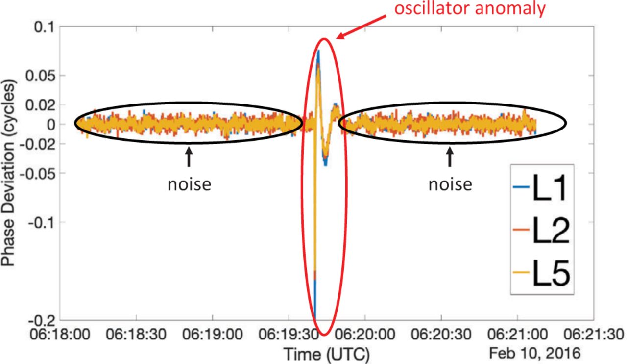
Feature set #2: Direct computation of the ratios may be affected by the presence of noise. Although each event is three minutes long, the actual event may only be present for ten seconds. The remaining time contains only noise, which does not follow the frequency dependency relationship. An example is shown in Figure 4. To mitigate this noise impact, phase deviations below a certain threshold are considered noise and excluded from the ratio calculation. In this feature set, a cutoff threshold of 0.05 cycles is used. The cutoff threshold can be applied to either frequency bands. For instance, we could apply the threshold to L1 or L2 when computing the ratio between L1 and L2. To fully utilize all information, we applied the threshold to both frequency bands, resulting in six ratios: L1 vs L2 with a threshold on L1, L1 vs L2 with a threshold on L2, L1 vs L5 with a threshold on L1, L1 vs L5 with a threshold on L5, L2 vs L5 with a threshold on L2, and L2 vs L5 with a threshold on L5.

Illustration of phase deviations of an oscillator anomaly event. The oscillator anomaly only shows up for ∼10 seconds; the rest only contains noise
Feature set #3: Similar to feature set #2, a lower cutoff threshold of 0.02 cycles is used to calculate the ratios.
3.2.2 Support vector machine #2
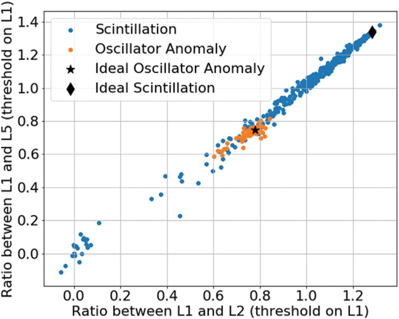
The above features are used as an input of the SVM #2 to detect the oscillator anomaly. Ideally, the features are linearly separable as there is a notable discrepancy between the ratios of these two events. For instance, Figure 5 shows the locations of ideal scintillation (black diamond) and oscillator anomaly (black star) in a 2D feature space. Here, only two features out of six are shown for the purpose of illustration. It’s very straightforward to draw a hyperplane to separate these two classes if the real samples are clustered around the corresponding ideal locations. In reality, however, the scintillation events may not follow the inverse proportion relationship. Noise in the signal and effects due to other processes and error sources introduce randomness and lead to deviations of measurements from the relationship. In addition, strong scintillation may lead to loss-of-lock and carrier-cycle slips and produce non-physical phase deviations in the phase measurements. These deviations make the detection problem more challenging. It is clear from Figure 5 that scintillation events are not only located on the upper right side of the oscillator anomaly but also extend to the lower left side. This makes the classification a non-linearly separable problem. Even with a 6D (instead of 2D) feature space, it’s still a non-linearly separable problem. That is the reason why we need to use an RBF kernel in SVM #2 to tackle this non-linearly separable problem.

Demonstration of scintillation and oscillator anomaly in feature space. Here, threshold = 0.02 is applied to compute the ratios. For illustration purposes, two ratios are presented here (L1 vs L5 with a threshold on L1 and L1 vs L5 with a threshold on L1). Ideal locations of scintillation and oscillator anomaly in the feature space are shown as a black diamond and black star, respectively. Examples of locations of real scintillation and oscillator anomaly samples are indicated as blue and orange circles, respectively
3.3 Stage 3: Satellite oscillator anomaly detection
The oscillator anomaly detected through the stage 2 algorithm can be due to either satellite or receiver oscillator anomalies. This third stage aims to differentiate satellite oscillator anomaly from a receiver oscillator anomaly. A receiver oscillator anomaly should simultaneously show up on measurements from multiple satellites in view, while a satellite oscillator anomaly is only present on the measurements from that particular satellite. As a result, measurements from multiple satellites are employed. A receiver oscillator anomaly is identified if multiple satellites simultaneously observe the oscillator anomaly; otherwise, it is a satellite oscillator anomaly. Of course, we can further confirm a satellite oscillator anomaly if it is simultaneously observed by multiple receivers (Ramesh et al., 2017).
4 PERFORMANCE EVALUATION OF STAGE ALGORITHM ON OSCILLATOR ANOMALY DETECTION
Extensive performance evaluation of phase disturbance detection (stage 1) can be found in Jiao et al. (2017). It has a reported accuracy of 92%. The differentiation between satellite and receiver oscillator anomalies (stage 3) is a trivial process. Therefore, we focus on the performance evaluation of the oscillator anomaly detection (stage 2) in this section.
4.1 Dataset description and evaluation method
In this work, we used measurements from GPS PRN1 and PRN25 collected at multiple stations around the world (Alaska, Ascension Island, Greenland, Hong Kong, Peru, Puerto Rico, Singapore) to construct the datasets. This is because these two satellites broadcast triple-frequency signals. Septentrio PolaRx5S receivers are deployed to collect 100 Hz phase measurements as the observables. The phase measurements are partitioned into three-minute sequential blocks without overlap, where each block is considered as one event (Jiao et al., 2017). In total, we detected 602 scintillation events and 126 oscillator anomalies from the dataset. In this study, the detected event labels are identified by visual inspection.
To evaluate the performance, 70% of samples in the dataset are randomly selected for training, and the rest are used for testing. The best hyperparameters are obtained via cross-validation (Bishop, 2006). It should be noted that the randomness in training/testing data selection also has an impact on the performance. To mitigate this impact, ten different arrangements for training/testing data splits are obtained and evaluated individually. The mean and standard deviation of the accuracy over these ten trials are used as the evaluation metric. The following metrics are also obtained for thorough performance assessments:
True positive rate (TPR). TPR measures the percentage of actual positive samples (oscillator anomaly in our case) that are correctly classified as positive. TPR is also known as the recall.
False positive rate (FPR). FPR measures the proportion of non-anomaly samples that are incorrectly classified as an anomaly.
Positive predictive value (PPV). PPV measures the proportion of predicted positive samples that are actual positive samples. PPV is also known as precision.
F1 score. It is a metric that combines TPR (recall) and PPV (precision) and is defined as the harmonic mean of both terms:

F1 score reaches its best value at one and worst at zero. It conveys the balance between recall and precision and is usually used to evaluate the model performance given an imbalanced dataset, as is the case in this study.

4.2 Performance evaluation of proposed RBF SVM
In Table 1, the detection performance using the proposed RBF SVM (SVM #2) with different feature sets is presented. Feature set #3 shows the best performance for all metrics. Feature set #1 has a slightly worse performance compared to feature set #3 because #3 employs a reasonable cutoff threshold to mitigate the noise impact on ratio calculation. The larger cutoff threshold used by feature set #2 dramatically degrades the detection performance. This is because a large cutoff threshold also excludes useful information for ratio calculation.
Performance evaluation of the proposed RBF SVM. Ten different training/testing splits are used. The mean and standard deviation (SD) of the metrics are shown. TPR denotes true positive rate; FPR denotes false positive rate; PPV denotes positive predictive value
For feature set #3, an average detection accuracy of 98.4% is obtained. The corresponding standard deviation is 0.5%, indicating that the algorithm performance is very stable under different training/testing splits. This also corroborates that the dataset is large enough to offer a robust performance. The TPR is 93.8%, which shows that the probability of missed detection of clock anomaly is 6.2%. The FPR is 0.7%, which demonstrates a very low probability of false alarm. The PPV is 97.1%, indicating that 2.9% of detected clock anomalies are actually scintillation events. Finally, the F1 score is 95.3%, showing a good classification performance in this imbalanced dataset.
4.3 Performance comparison
The proposed RBF SVM is also compared to the threshold method, the linear SVM, the threshold voting, and the logistic regression. A brief summary of these four methods is listed below:
Threshold Method: This method uses the ratio of phase deviations between L1 and L2 with a threshold on L1 as the only feature. A threshold is set such that any events with a ratio above the threshold are identified as scintillation and vice versa. In the training stage, a brute-force search algorithm is used to find the optimal threshold. Here, the optimal threshold is the one that gives the best performance in the training dataset. Thereafter, data in the testing dataset is classified based on this optimal threshold. Note that only the ratio between L1 and L2 in the proposed feature set is used.
Linear SVM: This method uses a linear kernel for SVM. Its decision boundary is linear.
Threshold Voting: The threshold method in 1) only applies the threshold on a single ratio. Threshold voting applies the threshold on all six ratios, where six independent classifications are conducted by applying the threshold method on each ratio. The final decision is made by majority voting. Tie is broken randomly.
Logistic Regression: This method uses a logistic function to conduct binary classification tasks. The decision boundary is also linear.
As shown in Table 2, the threshold method performs the worst in general. This is because the threshold method only utilizes the information from a single ratio and hence fails to benefit from ratio diversity. Based on the metric of accuracy, linear SVM, threshold voting, and logistic regression perform equally well. However, logistic regression has the lowest probability of missed detection of clock anomaly (highest TPR), followed by linear SVM. Threshold voting has the worst performance on missed detection of clock anomaly. In return, it has the best FPR (1.8%) and PPV (90.3%). These observations demonstrate that threshold voting has a smaller number of false positives (scintillation events that are wrongly classified as clock anomaly) given the same number of samples to be classified. If a lower false alarm rate is desired, threshold voting is preferred.
Performance comparison between the proposed RBF SVM, linear SVM, threshold method, threshold voting, and logistic regression. Ten different training/testing splits are used. The mean and standard deviation (SD) of the metrics are shown. TPR denotes true positive rate; FPR denotes false positive rate; PPV denotes positive predictive value
Finally, the proposed method RBF-based SVM with feature set #3 shows the best performance on all metrics except the TPR. The TPR is slightly worse than that for the logistic regression. However, it has a better accuracy, FPR, PPR, and F1 score with notable margins. As a result, the proposed RBF SVM is the best classifier among these algorithms.
5 PRELIMINARY DETECTION RESULTS USING THE RBF-BASED SVM METHOD WITH FEATURE SET #3
The accurate detection performance indicates that the proposed approach can be applied to automatically detect a satellite oscillator anomaly. In this study, we apply the proposed approach to a database obtained by our global network of GNSS monitoring stations in 2017 and 2018, where Septentrio PolaRx5S receivers are deployed to collect 100 Hz phase measurements (Jiao, 2017). Station locations include Alaska, Greenland, South Korea, Puerto Rico, and Chile. All GPS block IIF satellites are processed, including PRN1, PRN3, PRN6, PRN8, PRN9, PRN10, PRN24, PRN25, PRN26, PRN27, PRN30, and PRN32. Table 3 shows the data availability at these stations. It should be noted that we differentiate between satellite and receiver oscillator anomaly by checking whether the same oscillator anomaly is observed by all satellites in view at the same time. Cross-validation by multiple nearby receivers was performed in an earlier study and demonstrated the robustness of the method (Liu & Morton, 2019). A more comprehensive evaluation using cross-validation of multiple nearby receivers will be conducted in a future work. Furthermore, the purpose of these preliminary detection results is to demonstrate that the proposed RBF-based SVM method is capable of automatically conducting satellite oscillator anomaly detection given a large volume of data. A comprehensive global characterization of GPS satellite oscillator anomaly (including both block IIRM and block IIF) is currently underway and is the subject of a future publication.
Availability of processed data
An example of the detected oscillator anomaly is illustrated in Figure 6. Because of the frequency dependency property, the L1 band shows the largest phase deviation, while the L5 band shows the smallest. The maximum phase deviation at the L1 band reaches a magnitude of approximately 0.18 cycles.
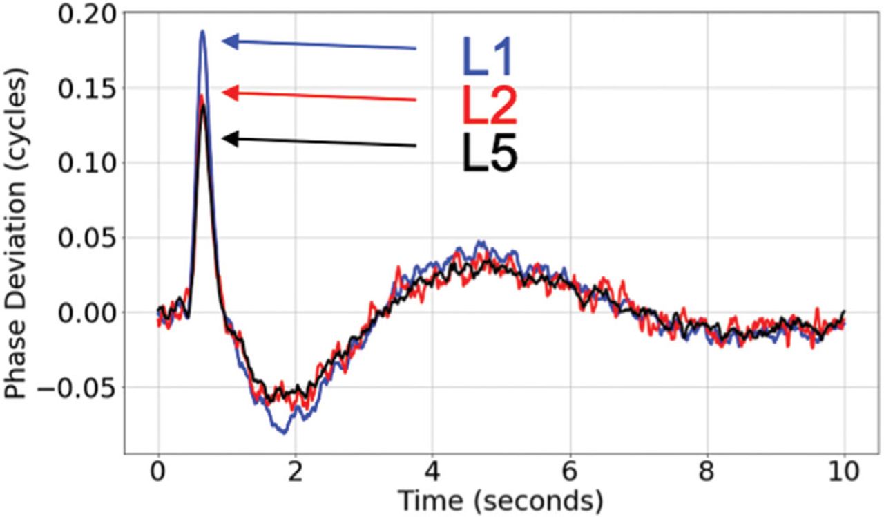
An example of satellite oscillator anomaly
To obtain the statistics of maximum phase deviation at L1, a histogram for all detected oscillator anomalies is shown in Figure 7. It is clear that most of the detected oscillator anomalies have a maximum phase deviation at L1 of around 0.2 cycles. Given the magnitude of the maximum phase deviation, these are considered small oscillator anomalies.

Histogram of L1 maximum phase deviation
The station-by-station statistics of detected oscillator anomaly events on GPS block IIF satellites are shown in Table 4. There are around two daily oscillator anomaly events observed from each station. The Alaska station has the highest average number of observations (3.4/day), and the South Korea and Chile stations show the lowest average number of observations (1.7/day).
Station-wise statistics of detected oscillator anomaly events on GPS block IIF satellites
To further investigate how different satellites behave, a histogram for each satellite’s average oscillator anomaly observations per visible day per station is shown in Figure 8. Here, a visible day refers to a 24-hour period during which the corresponding satellite is in view with elevation above 20° at the station. In general, the most frequent oscillator anomaly is observed from PRN 10, followed by PRN 26, PRN 1, PRN 3, PRN6, and PRN9. Very few oscillator anomaly events are observed from PRN 8, PRN 24, PRN 25, PRN 27, PRN 30, and PRN 32. The Alaska station usually observes frequent oscillator anomaly events from PRN1, PRN9, PRN10, and PRN 26. In particular, approximately five oscillator anomalies per visible day can be seen from PRN10 at Alaska.
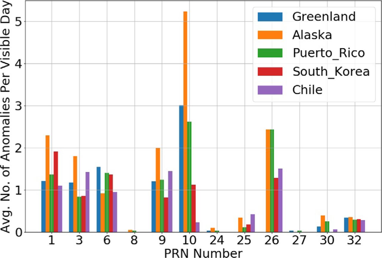
Satellite-wise average number of detected oscillator anomaly events per visible day at each station
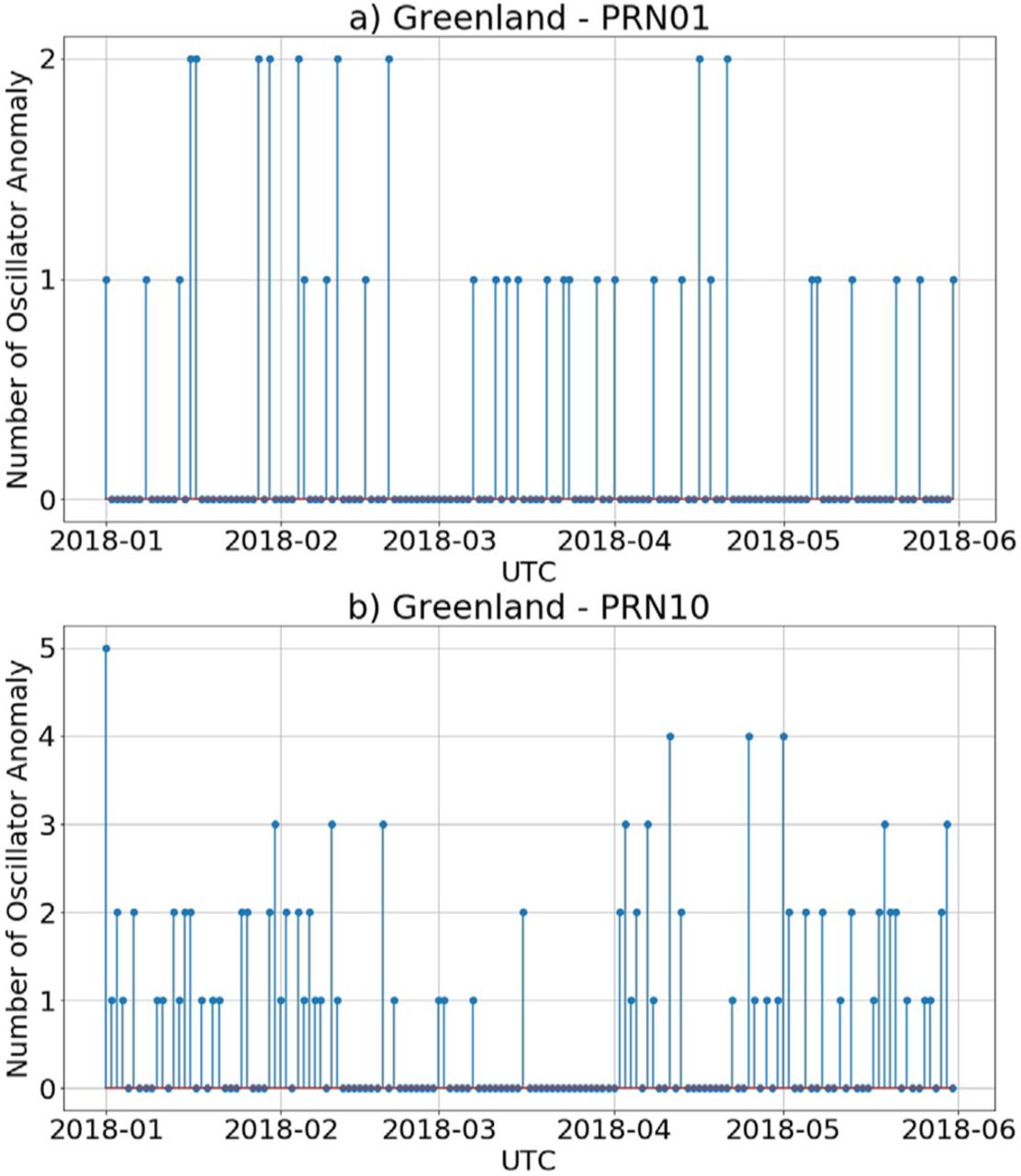
We also investigate the time series of the satellite oscillator anomaly occurrence. The oscillator anomaly daily occurrence over Greenland is shown in Figure 9. Random occurrence patterns are obtained from both satellites. This observation indicates that the oscillator anomaly events do not occur periodically.

Satellite oscillator anomaly daily occurrence over Greenland. a) PRN1; b) PRN10
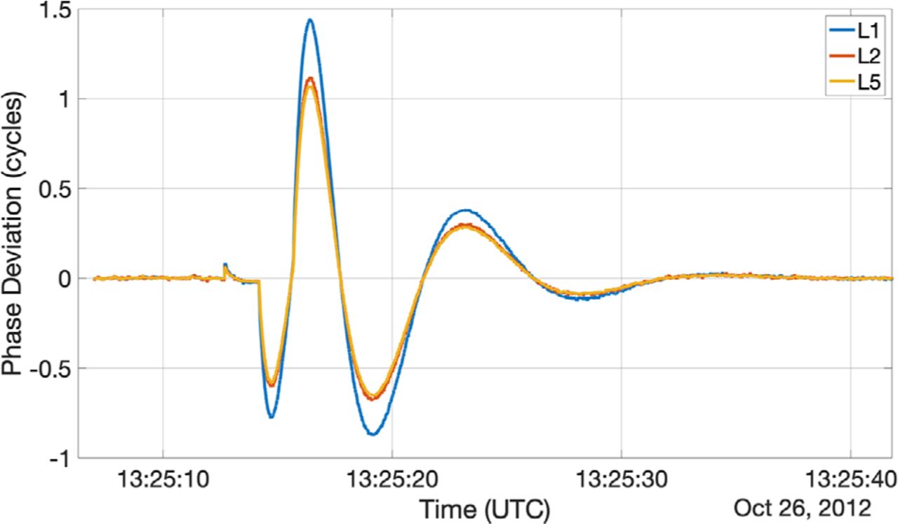
The results above demonstrate that the proposed method is capable of detecting small oscillator anomalies. To investigate how well the method performs on large oscillator anomaly events, we apply the proposed method to process the data on October 26th, 2012, on which day the authors in Benton and Mitchell (2014) observed several large satellite oscillator anomaly events. As shown in Table 5, eight large oscillator anomaly events are detected by our method, which matches with the observations in Benton and Mitchell (2014). An example of the large oscillator anomaly is shown in Figure 10. The maximum phase deviation at the L1 band reaches a magnitude of approximately 1.5 cycles. This result shows that the proposed method can also detect large oscillator anomalies. The reason that the proposed method can detect both small and large oscillator anomalies is because the features are based on the ratios of phase deviations between different frequency bands rather than the magnitude.
Summary of Detected Satellite Oscillator Anomaly

An example of large satellite oscillator anomaly observed on October 26th, 2012 from PRN1
6 CONCLUSION AND FUTURE WORK
We designed an RBF SVM to differentiate the oscillator anomaly from ionospheric scintillation in a dataset that has carrier-phase disturbances. The RBF kernel enables SVM to construct a nonlinear decision boundary and, thus, shows the best performance. Three different feature sets are proposed, and the feature set #3 shows superior performance because it mitigates the noise impact on ratio calculation. The RBF SVM with this feature set has a detection accuracy of 98.4%. In addition, by incorporating this RBF SVM, the proposed approach is applied on a database to conduct automatic satellite oscillator detection. The preliminary detection results corroborate that the proposed approach has the potential to be deployed on global satellite oscillator anomaly monitoring systems.
In the future, the proposed approach can be extended to detect the satellite oscillator anomaly on GNSS satellites with dual-frequency signals and with data collected at lower rates. Furthermore, global detection and characterization of the satellite oscillator anomaly events can be conducted.
The proposed detection method in stage 2 can only distinguish between the oscillator anomaly and scintillation. As another common error source, multipath could also cause disturbance. An elevation mask (30°) is applied to mitigate multipath in this work. In the future, multipath can be added as an additional class in the detection method, which could distinguish among the oscillator anomaly, scintillation, and multipath.
HOW TO CITE THIS ARTICLE
Liu Y, Morton YJ. Automatic detection of ionospheric scintillation-like GNSS satellite oscillator anomaly using a machine-learning algorithm. NAVIGATION. 2020;67:651–662. https://doi.org/10.1002/navi.385
ACKNOWLEDGEMENT
This work is supported by the Space Weather Technology, Research and Education Center (SWxTREK), University of Colorado at Boulder, a grant from NASA (#NNX15AT54G), and a contract from Lockheed Martin. The authors are grateful for Mr. Ian Collett and Rachael Morton for their valuable comments and suggestions on the manuscript. The data used in this study is collected at the global ionospheric scintillation monitoring network established by the Satellite Navigation and Sensing (SeNSe) Lab at the University of Colorado Boulder.
Footnotes
Funding information
Space Weather Technology, Research and Education Center (SWxTREK), University of Colorado, Grant/Award Number: #NNX15AT54G
- Received December 30, 2019.
- Revision received April 17, 2020.
- Accepted June 7, 2020.
- © 2020 Institute of Navigation
This is an open access article under the terms of the Creative Commons Attribution License, which permits use, distribution and reproduction in any medium, provided the original work is properly cited.


Jump to section
- Article
- Abstract
- 1 INTRODUCTION
- 2 SUPPORT VECTOR MACHINE
- 3 SATELLITE OSCILLATOR ANOMALY DETECTION
- 4 PERFORMANCE EVALUATION OF STAGE ALGORITHM ON OSCILLATOR ANOMALY DETECTION
- 5 PRELIMINARY DETECTION RESULTS USING THE RBF-BASED SVM METHOD WITH FEATURE SET #3
- 6 CONCLUSION AND FUTURE WORK
- HOW TO CITE THIS ARTICLE
- ACKNOWLEDGEMENT
- Footnotes
- REFERENCES
- Figures & Data
- Supplemental
- References
- Info & Metrics
Related Articles
Cited By...
- No citing articles found.