

Abstract
Prior work established a model for uncertain Gauss-Markov (GM) noise that is guaranteed to produce a Kalman filter (KF) covariance matrix that overbounds the estimate error distribution. The derivation was conducted for the continuous-time KF when the GM time constants are only known to reside within specified intervals. This paper first provides a more accessible derivation of the continuous-time result and determines the minimum initial variance of the model. This leads to a new, non-stationary model for uncertain GM noise that we prove yields an overbounding estimate error covariance matrix for both sampled-data and discrete-time systems. The new model is evaluated using covariance analysis for a one-dimensional estimation problem and for an example application in Advanced Receiver Autonomous Integrity Monitoring (ARAIM).
SUMMARY OF MAIN RESULT
Let 𝚺 be the Kalman filter (KF) estimate error covariance matrix and 𝐏 be the true estimate error covariance matrix. The inequality 𝚺 ≥ 𝐏 means that the predicted variance 𝜶𝑇𝚺𝜶 is greater than or equal to the true variance 𝜶𝑇𝐏𝜶 for any real vector 𝜶.
Suppose that the measurement and process noise components are known to be first-order Gauss-Markov random processes (GMPs). These processes are completely specified by a time constant 𝜏, steady-state variance 𝜎2 and initial variance  , and propagate according to the difference equation

where 𝑘 is an arbitrary time index, Δ𝑡 = 𝑡𝑘+ 1 −𝑡𝑘 is the discrete-time sampling interval, WGN(0, 1) indicates zero-mean white Gaussian noise with unit variance and 𝑁(0,  ) denotes a zero-mean normal random variable with variance
  .
.
When 𝜏 and 𝜎2 are only known to reside in the intervals [𝜏min,𝜏max] and  , a state-augmented KF that models 𝑎𝑘 with

is guaranteed to produce a covariance matrix 𝚺 ≥ 𝐏.
1 INTRODUCTION
Safety-critical GNSS applications must ensure that the probability of the estimate error exceeding predefined bounds is acceptably small. This probability is often referred to as integrity risk. In aviation navigation applications, cumulative distribution function (CDF) overbounding has been used extensively over the past 10-20 years to derive upper bounds on integrity risk for snapshot least-squares, GPS-based navigation (DeCleene, 2000; Rife et al., 2004, Rife et al., 2006; Blanch et al., 2019). However, state estimation using a recursive filter can be more accurate and enables integration with additional sensors like an inertial measurement unit (IMU). One challenge with sequential estimation is how to conservatively account for time-correlated noise like GPS multipath. Precise multipath models are very difficult to obtain, as illustrated in Pervan et al. (2017), for an ensemble of empirically derived multipath autocorrelation functions (ACFs). Thus, even using the best models available, there is uncertainty when dealing with time-correlated noise.
Existing CDF overbounding methods do not account for model uncertainty over time, which has prompted the development of new techniques. Theoretical approaches were developed in (Rife & Gebre-Egziabher, 2007; Pulford, 2008) to bound the integrity risk of linear systems driven by a spherically symmetric random process. The authors in Langel et al. (2014) derive an integrity risk bound for the KF when measurement and process noise are Gaussian with ACFs that are unknown but can be upper- and lower-bounded. The methods in (Rife & Gebre-Egziabher, 2007; Pulford, 2008; Langel et al., 2014) are attractive because they do not require any knowledge about the mathematical form of the input noise ACFs. However, the price to pay is that (Rife & Gebre-Egziabher, 2007; Pulford, 2008; Langel et al., 2014) all provide a batch solution in the sense that they require storing matrices whose dimensions grow without bound at a rate dictated by sensor sampling rates. For real-time applications, these techniques are only suitable for short duration applications. If high-rate sensors like an IMU are being used, the maximum allowable duration could be on the order of minutes before computational and memory constraints begin to prohibit real-time operation. One way to derive a practical algorithm is to stipulate that the measurement and process noise ACFs are known up to a finite set of uncertain parameters.
State estimation with uncertain parameters has been studied extensively in the robust estimation literature. Guaranteed cost filtering emerged in the 1990s as a technique for defining a robust filter whose estimate error variance is guaranteed to be smaller than a given bound. These filters often require determination of one or more scale parameters using an optimization algorithm and can display unstable behavior. Dependence on scale parameters and questionable stability characteristics means that significant effort is required up front to design the estimator. Real-time capability is also a challenge, given the need to numerically solve an optimization problem. For these reasons, robust estimators have not been widely adopted so far by the navigation community to upper bound KF integrity risk when the input noise ACFs are uncertain.
This paper builds on the work in Tupysev et al. (2009), where a guaranteed upper bound on the KF estimate error variance is derived when process and measurement noise components are first-order GMPs with unknown, but bounded, time constants. Reference Tupysev et al. (2009) shows that in order to guarantee that the KF covariance matrix overbounds the estimate error, both the minimum and maximum time constants must be used in the KF matrices. The derivation is conducted for the continuous-time KF, and a covariance analysis is performed for an IMU-aided navigation problem to show that the estimate error variance is bounded. The authors in Tupysev et al. (2009) indicate that the initial variance of their model must be inflated relative to the true GM variance but do not specify how much inflation is necessary. They also did not discuss how their results apply for the more common case of discrete-time systems. We will address both deficiencies.
The paper begins with the problem statement and motivation for its study in Sections 2 and 3. Starting from a sampled-data system model, Sections 4 through 5.1 provide a more accessible derivation of Equation (23) in Tupysev et al. (2009), following many of the authors’ key developments. In Section 5.2, we derive the minimum initial variance for the GM model (Equation (25)) that yields an overbounding covariance matrix for the mixed continuous-discrete KF. This expression is a previously unknown result that leads to a new, non-stationary model for GM noise that we prove in Section 5.3 results in an overbounding estimate error covariance matrix for the discrete-time KF. The proof is a new development that rigorously justifies using our model to account for uncertain GM noise in a discrete-time setting. An illustrative example shows that the non-stationary model provides a significantly tighter bound on the estimate error variance compared to a stationary model.
One application where time-sequential estimation is being explored for high integrity navigation is Vertical Advanced Receiver Autonomous Integrity Monitoring, or V-ARAIM, which seeks to provide worldwide vertical guidance of aircraft using dual-frequency measurements from GPS and Galileo. It was shown recently that V-ARAIM performance can be significantly improved by processing time-sequences of measurements (Joerger & Pervan, 2015, 2016). In Section 6, we carry out a performance analysis for time-sequential V-ARAIM. Multipath and residual tropospheric errors are first-order GMPs with time constants that reside within their own specified intervals. We use our new GM model to establish global availability maps that show sequential V-ARAIM outperforms traditional snapshot ARAIM even though the multipath and residual tropospheric error time constants are uncertain. Concluding remarks and suggestions for future study are given in Section 7.
2 PROBLEM SETUP
Consider the state estimation problem for the sampled-data system
 1
1
where 𝝃 ∈ ℝ𝑛 is the state vector, 𝒛𝑘 ∈ ℝ𝑚 is the measurement vector and 𝒘(𝑡) ∈ ℝ𝑝, 𝒗𝑘 ∈ ℝ𝑠 are the process and measurement noise vectors, respectively. The matrices 𝐀, 𝐁, 𝐂𝑘 and 𝐃𝑘 are known and of appropriate dimension.
A sampled-data system model is used for most of the theoretical development in this paper because many systems encountered in practice are described by Equation (1). State dynamics are often derived from physical laws (e.g., Newton’s laws of motion) and take the form of continuous-time differential equations, whereas external measurements of a system are usually taken with digital sensors. Recognizing that Equation (1) is typically converted entirely to discrete-time prior to developing an estimator, results for sampled-data systems are extended to discrete-time systems in Section 5.3.
The vectors 𝒘 and 𝒗𝑘 are known to be linear combinations of a first-order GMP vector 𝒂 ∈ ℝ𝑙 and zero-mean WGN vectors 𝒏(𝑡) ∈ ℝ𝑝 and 𝒓𝑘 ∈ ℝ𝑠. That is
 2
2
such that 𝐄w(𝑡) ∈ ℝ𝑝×𝑙 and 𝐄v,𝑘 ∈ ℝ𝑠×𝑙 are known matrices, 𝐍(𝑡) ∈ ℝ𝑝×𝑝 is the power spectral density matrix of 𝒏(𝑡), 𝐑𝑘 ∈ ℝ𝑠×𝑠 is the covariance matrix of 𝒓𝑘 and 𝛿(𝑡), 𝛿kl are the Dirac delta function and Kronecker delta, respectively. 𝐍(𝑡) and 𝐑𝑘 are unknown, but we assume that  and
and  can be determined.
For the GMP vector 𝒂, 𝐋 and 𝐔 are (Gelb et al., 1974)
 3
3
where  and 𝜏𝑖,𝑖 = 1,…,𝑙 are only known to reside in specified intervals. The goal of the paper is to develop a KF whose predicted estimate error covariance matrix accounts for uncertainty in
  and 𝜏𝑖. In subsequent sections, “(𝑡)” will be omitted to lighten the notation.
State augmentation (Anderson & Moore, 1974) is commonly used to account for correlated noise and involves appending 𝒂 to 𝝃 to form the new linear system
 4
4
With 𝒙𝑇 = [𝝃𝑇 𝒂𝑇], Equation (4) can also be written as
 5
5
Equation (5) is a linear system driven by zero-mean WGN. Thus it is permissible to estimate 𝒙 using a KF. Since  and 𝜏𝑖 are unknown, it is not clear what values should be used to define the KF. One criterion is to use parameter values so the predicted estimate error distribution overbounds the true error distribution over the range of admissible values.
To define an overbounding distribution, let  be an estimate of a specified state 𝑦 and define
  as the associated estimate error. Then for a maximum tolerable error 𝓁𝑦, an overbounding distribution is one that produces an upper bound on the integrity risk 𝑃(|𝜀𝑦| ≥ 𝓁𝑦). Given that Equation (5) is a linear system driven by zero-mean WGN and the fact that the KF is a linear unbiased estimator, it follows that
  . In this case, an upper bound on integrity risk is equivalent to an upper bound on the estimate error variance
  . Therefore, subsequent sections of the paper will focus on developing an upper bound on the estimate error variance for any state of interest.
3 MOTIVATIONAL EXAMPLE
Before developing a rigorous approach for defining an overbounding distribution in the presence of uncertainty, it is instructive to address the fallacies in current thinking. The conventional wisdom is that a KF using upper bound parameter values will produce an estimate error covariance matrix that overbounds the true error distribution. We use a simple one-dimensional estimation problem to demonstrate that this heuristic is not always accurate.
Consider the vehicle in Figure 1 moving at constant speed 𝑢 along the 𝑥-axis from an initial point 𝑝0. Noisy measurements of the current position are available, described by the model
 6
6
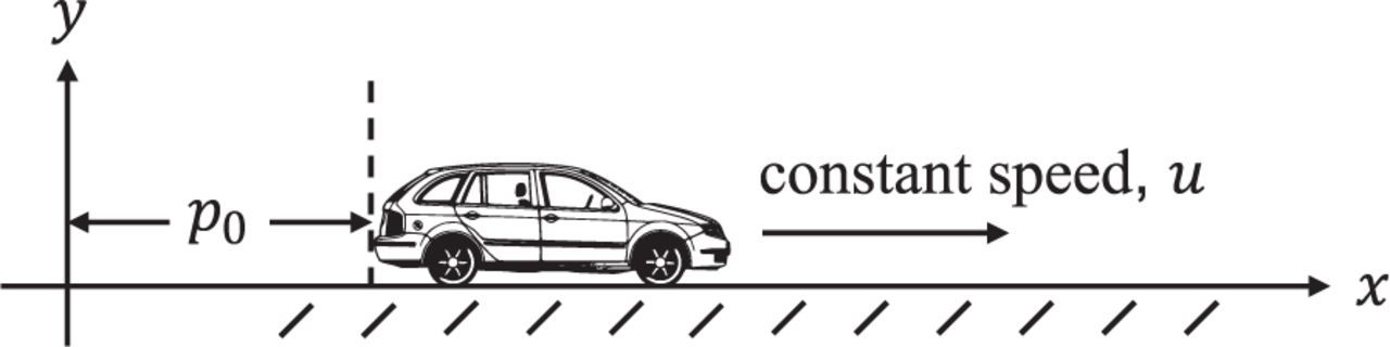
One-dimensional position and velocity estimation
where 𝑣𝑘 is the sum of a first-order GMP and zero-mean WGN. That is, 𝑣𝑘 = 𝑎𝑘 +𝑟𝑘 such that  and
and
 7
7
The variances are known and given by  and
and  . However, the time constant 𝜏 is only known to lie in the interval [10,100] s. Noting that 𝑝0 and 𝑢 are constants, state augmentation results in the estimation problem
 8
8
such that the initial estimate error covariance matrix 𝐏0 is diagonal with nonzero elements: [10 m2,1m2∕s2,1m2].
The KF is constructed assuming that 𝜏 = 100 seconds. However, suppose that 𝜏 is actually equal to 50 seconds. We want to compare the KF’s predicted estimate error variance to the true variance in this case. The true estimate error variance is obtained through Monte Carlo simulation. Measurements of current position are generated according to the true measurement model and passed into the KF. The variance is then estimated from the sample estimate error distribution. We saw that the change in estimated variance between 800,000 trials to one million trials was indistinguishable. Thus, one million trials is sufficient to accurately determine the true variance.
Figure 2 shows the estimate error standard deviation predicted by the KF minus the true standard deviation for the initial position and speed states. One might expect to see that the estimated-minus-true difference is positive at all times when assuming that 𝜏 = 𝜏max. This is clearly not the case. For the initial position state, the assumption that 𝜏 = 𝜏max is eventually conservative after 60 seconds have elapsed. For the speed state, assuming that 𝜏 = 𝜏max always leads to optimistic predictions of the estimate error standard deviation. This simple example demonstrates that a more rigorous approach is needed to establish an overbounding estimate error distribution when correlated measurement error models are uncertain.
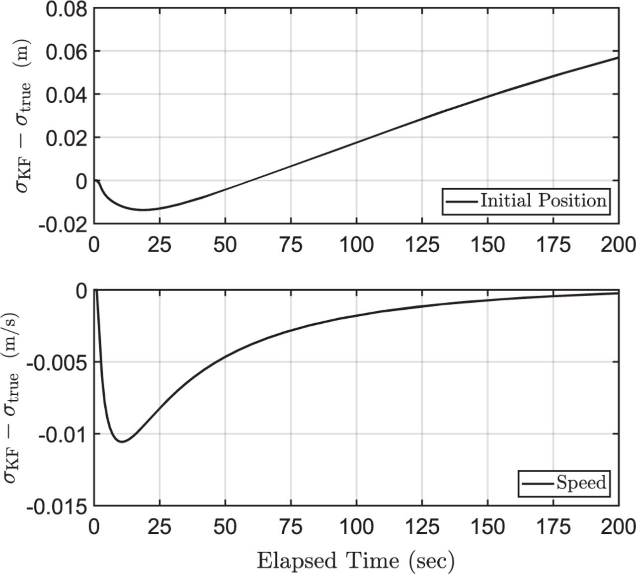
Difference between predicted and true estimate error standard deviations for a KF that assumes 𝜏 = 𝜏max
4 TRUE COVARIANCE MATRIX
This section derives propagation equations for the true estimate error covariance matrix when the KF uses models that do not correspond to the actual process and measurement noise statistics. In what follows, the notation (⋅)𝑘|𝑘 will be used to denote a quantity at time index 𝑘 based on all measurements up to and including time index 𝑘. The KF for the system in Equation (5) is defined by the recursion
 9
9
The filter designer must specify  (which is contained in
  ) and
) and  . These matrices generally will not describe the true measurement and process noise statistics because the parameters defining them are uncertain. The KF covariance matrix
  therefore does not accurately capture the true estimate error distribution, and a new covariance matrix 𝐏 must be defined that accounts for model uncertainty.
When  , Appendix A shows that the KF estimate error vector
  propagates according to
  , where
  . Thus, 𝜺 and 𝒂 must be considered simultaneously when determining the true covariance matrix for 𝜺. The correlation between 𝜺 and 𝒂 is properly accounted for by forming the augmented vector 𝒆𝑇 = [𝜺𝑇 𝒂𝑇]. This method of accounting for model uncertainty is similar to the approach in Gelb et al. (1974). The only difference is that we focus on uncertainty in 𝐋, whereas Gelb et al. (1974) considers uncertainty in the entire transition matrix 𝐅. Appendix A shows that 𝐏 = 𝐸[𝒆𝒆𝑇] evolves according to
 10
10
such that
 11
11
Equations (10) and (11) contain both true and estimator matrices and thus reflect that 𝐍, 𝐑, 𝐔 and 𝐅 are uncertain. For example,  and
and  go into determining 𝐊𝑘, but 𝐍 and 𝐑𝑘 also appear explicitly. However, 𝐏 cannot be computed in practice because of the unknown matrices involved. We therefore seek to define a covariance matrix 𝚺 free of dependence on unknown matrices such that (𝚺 − 𝐏) ≥ 0, that is, 𝚺−𝐏 is positive semi-definite. This criterion ensures that the predicted error variance for any state is an upper bound on the true variance.
5 MODELING UNCERTAIN GM NOISE
The goal of this section is to define a propagation structure for 𝚺 and use the criteria (𝚺−𝐏) ≥ 0 to derive a model for uncertain GM noise. Following the approach in Tupysev et al. (2009), we stipulate that 𝚺 propagates in a manner similar to Equations (10) and (11), that is,
 12a
12a
 12b
12b
This structure was chosen because, as we will see, it enables  ,
,  and the initial covariance matrix 𝚺(0) to be defined explicitly from the requirement (𝚺 − 𝐏) ≥ 0. The covariance error matrix 𝚫 = 𝚺−𝐏 propagates as
 13a
13a
 13b
13b
Equation (13a) is a matrix differential equation with initial condition 𝚫𝑘−1|𝑘−1 and whose solution at 𝑡 = 𝑡𝑘 is 𝚫𝑘|𝑘−1. The matrix 𝚫𝑘|𝑘−1 is positive semi-definite if 𝚫𝑘−1|𝑘−1 ≥ 0 and  (see Dieci & Eirola, 1994). The quadratic structure in Equation (13b) ensures that 𝚫𝑘|𝑘 ≥ 0 when 𝚫𝑘|𝑘−1 ≥ 0 and
  Therefore, we must have an initial matrix 𝚫(0) ≥ 0 and
  to guarantee that 𝚫(𝑡) ≥ 0 for all 𝑡.
5.1 Continuous-time model
We will now provide a more accessible derivation of the continuous-time model for uncertain GM noise given in Tupysev et al. (2009), following many of the authors’ key developments. In preparation for the first step, defining  readers should re-familiarize themselves with the definitions in Equation (3).
Let  formed with the upper bound values for
  and the lower bound values for 𝜏𝑖. Let’s also define
  as the matrix 𝐔 populated with the true time constants 𝜏𝑖 and as yet undetermined variances
  . Then with
  defined as
 14
14
it is clear that  for all admissible values of
  and 𝜏𝑖. However,
  could never be constructed because it depends on the unknown matrix
  . Therefore, we must use a mathematical approach to make 𝚺 insensitive to
  . To see how this can be accomplished, form the partitioned matrix
  so that Equation (12a) can be written in expanded form as
 15a
15a
 15b
15b
 15c
15c
where
 16
16
We are only interested in propagating 𝚺𝑥, the block of 𝚺 corresponding to 𝜺. In its current form, Equation (15a) cannot be propagated because it depends on the unknown matrix Δ𝐅. We can eliminate Δ𝐅 by forcing 𝚺𝑥𝑎(𝑡) = 𝟎 for all 𝑡. To achieve this, let  and impose the constraint
 17
17
which simplifies Equation (15b) to the unforced linear differential equation  . Next, set the initial condition 𝚺𝑥𝑎(0) = 𝟎. The only solution to an unforced linear differential equation with zero initial condition is the trivial solution. Therefore, it must be that 𝚺𝑥𝑎(𝑡) = 0 for all 𝑡, as desired.
Equation (17) has additional ramifications when we consider the alternative form 𝚺𝑎 = −(Δ𝐋)−1𝐔. The matrices Δ𝐋 and 𝐔 are time-invariant, which implies that  . Making the substitutions
  into Equation (15c) results in the additional constraint
 18
18
Noting that 𝐋, , 𝐔 and
  are diagonal matrices, Equation (18) is equivalent to the set of scalar conditions
 19
19
It is worth reiterating that 𝜏𝑖 and  are unknown,
  is a quantity we need to determine, and
  must be greater than or equal to
  . To determine
  , first solve Equation (19) for
  , resulting in
 20
20
We know that variances are never less than zero. The denominator in Equation (20) indicates that the only way to guarantee that  for any 𝜏𝑖 ∈ [𝜏𝑖,min,𝜏𝑖,max] is to set
  equal to 𝜏𝑖,max.
With  , the inequality in Equation (20) simplifies to 1 ≥ 𝜏𝑖∕𝜏𝑖,max, which is satisfied for all admissible values of
  . Thus, we satisfy the requirement that
  . Having determined the diagonal elements of
  and
and  , we can conclude that 𝚺𝑥 ≥ 𝐏𝑥 when first-order GMPs are modeled according to
 21
21
Equation (21) is identical to Equation (23) in Tupysev et al. (2009). This completes the proof of the main result in Tupysev et al. (2009). At this point, the model in Equation (21) is incomplete without specifying the initial variance. The reader also may be wondering about the role of  . It is comforting that
  is not required to propagate 𝚺𝑥 because its dependence on the unknown time constant 𝜏𝑖 means that
  can never be constructed. However, a previously unknown fact is that
  places constraints on the initial variance for the GM model. This new result is covered next.
5.2 Initialization
Reference Tupysev et al. (2009) indicates that the initial variance of the GM model must be inflated relative to the true variance but does not provide any insight as to how much inflation is required. In this section, we derive the tightest bound on the initial variance for the model in Equation (21) that still guarantees 𝚺𝑥 ≥ 𝐏𝑥.
Section 5.1 showed that the initial cross-covariance 𝚺𝑥𝑎(0) must be zero to eliminate any dependence of 𝚺𝑥 on the unknown matrix Δ𝐅. Assuming that 𝜺𝜉,0 and 𝜺𝑎,0 are initially uncorrelated with covariance matrices 𝚺𝜉,0 and 𝚺𝑎,0, the requirement 𝚺𝑥𝑎(0) = 𝟎 leads to the initial covariance matrix
 22
22
where 𝚺𝜉,0 is assumed to be known (e.g., from an initialization algorithm), 𝚺𝑎,0 is what we seek to define in this section, and  is a diagonal matrix populated with the
  in Equation (20).
Appendix B shows that the true initial covariance matrix is
 23
23
such that 𝐏𝑎,0 is a diagonal matrix comprised of the unknown variances  . We showed earlier that 𝚺(0) ≥ 𝐏(0) is a necessary condition to ensure that 𝚺(𝑡) ≥ 𝐏(𝑡) for all 𝑡. We assume that 𝚺𝜉,0 can be specified so that 𝚺𝜉,0 ≥ 𝐏𝜉,0. Then using the fact that a block diagonal matrix is positive semi-definite if and only if each diagonal block is positive semi-definite, 𝚺𝑎,0 must be specified so that
 24
24
Denoting an arbitrary diagonal element of 𝚺𝑎,0 as  , Appendix B shows that Equation (24) is satisfied if
 25
25
It is worth noting that the model in Equation (21) is stationary when initialized with a variance  that is greater than the lower bound in Equation (25). A stationary model for uncertain GMPs is appealing because GMPs are in fact stationary. However, by initializing with the minimum variance in Equation (25), it is possible to obtain a tighter bound on the estimate error variance using a non-stationary model. This will be demonstrated in Subsection 5.4 for the one-dimensional example considered in Section 3.
5.3 Discrete-time model
Even though Equation (1) may be the native description of a system, it is often converted entirely to discrete-time when designing and implementing a KF. We will prove in this section that the discretized form of Equation (21) yields an overbounding estimate error covariance matrix for the discrete-time KF.
Consider a discrete-time system analogous to Equation (4)
 26
26
where  and
and  . As before, we assume that
  and 𝚺𝜉,0 ≥ 𝐏𝜉,0 can be specified. Suppose that
  is estimated with a KF that models 𝒂𝑘 using the discretized form of Equation (21). From the continuous-to-discrete mapping (Rogers, 2003)
 27
27
with 𝜙 = 𝑒−Δ𝑡∕𝜏, the discretized form of Equation (21) is seen to be
 28
28
Following a similar approach to Subsection 5.1, Appendix C shows that the covariance error matrix 𝚫 = 𝚺−𝐏 for the discrete-time KF propagates as
 29a
29a
 29b
29b
Given that our analysis of sampled-data systems also considered discrete-time measurements, it is no surprise that Equation (29b) is identical to Equation (13b). However, Equation (29a) differs from the continuous version in Equation (13a) in that there is an additional matrix dependent on Δ𝐅𝑘 that must now be considered.
To show that 𝚫𝑘|𝑘 ≥ 0, first note that whether the original system is a sampled-data system or a discrete-time system, initialization is the same. Thus, the results from Subsection 5.2 also apply here, that is, initializing with 𝚺𝜉,0 ≥ 𝐏𝜉,0 and the variances in Equation (28) ensures that 𝚺0|0 ≥ 𝐏0|0. Second, notice that the quadratic structure in Equation (29b) guarantees that 𝚫𝑘|𝑘 ≥ 0 if 𝚫𝑘|𝑘−1 ≥ 0. Therefore, if we can establish that 𝚫𝑘+ 1|𝑘 ≥ 0, this will prove that the discrete-time KF covariance matrix overbounds the estimate error distribution.
Determining whether 𝚫𝑘+ 1|𝑘 ≥ 0 comes down to showing that
 30
30
which we prove is true in Appendix D. Hence, we can conclude that for a discrete-time system, the model given in Equation (28) yields a KF covariance matrix that overbounds the estimate error distribution when the GM time constants are uncertain.
5.4 Motivational example revisited
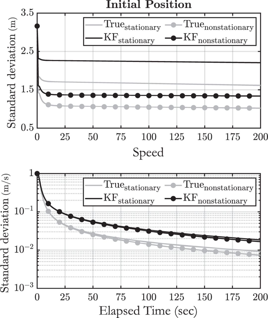
A visual representation of the paper’s main result is obtained by revisiting the motivational example from Section 3. The KF is run twice, once with the non-stationary model in Equation (28) and once with the stationary model where  . Just as before, the true estimate error variance is obtained through Monte Carlo simulation.
Figure 3 shows the estimate error standard deviation predicted by the KF and the true standard deviation using each model. The predicted standard deviation is always greater than the true standard deviation, indicating that both models provide an upper bound on the estimate error variance. For the speed state, there is almost no visible benefit of using the non-stationary model. However, the benefit is clear for the initial position state. Not only is the variance bound smaller using the non-stationary model compared to the stationary model, but it is also less conservative. That is, the gap between the predicted and true standard deviations is smaller when using the non-stationary model for GM noise.

KF standard deviation compared to truth when using stationary and non-stationary bounding GMP models
Remember that 𝚺 was derived so that 𝚺 ≥ 𝐏. This means that the ellipsoid corresponding to 𝚺 circumscribes the ellipsoid associated with 𝐏 for any admissible 𝜏. Figure 4 shows the true covariance matrix obtained from Monte Carlo simulation in gray and the KF covariance matrix in black, at an elapsed time of 10 seconds, when using the stationary and non-stationary bounding models. The true covariance matrices are different for each bounding model because they are obtained using two separate estimators, derived from two different values for the initial GM state variance. We can see that the KF covariance ellipse does indeed circumscribe the true ellipse. The white space between 𝐏 and 𝚺 along the 𝑥-axis is smaller for the non-stationary bound, and about the same for both bounds along the 𝑦-axis. This reiterates the conclusion from Figure 3 that the non-stationary bound is tighter than the stationary bound for the initial position state, but provides little benefit for the speed state.

True and bounding covariance ellipses for the motivational example in Section 3. Ellipses are shown at an elapsed time of 10 seconds
The ability to overbound the estimate error distribution for any linear combination of state vector components is critical for certain applications. In aircraft precision navigation, for example, horizontal integrity risk assessment requires overbounding a combination of the north and east components of positioning error. For the first time, the methods developed in this paper provide a practical means to determine such an overbound in the presence of uncertain GM noise. The next section will implement the non-stationary model in an example application of aircraft navigation using ARAIM (Working Group C - ARAIM Technical Subgroup, 2012, 2015, & 2016).
6 APPLICATION TO SEQUENTIAL ARAIM PERFORMANCE ANALYSIS
The baseline ARAIM algorithm is a “snapshot” implementation that uses dual-frequency multi-constellation measurements at one time-instant to achieve LPV-200 requirements, that is, requirements for localizer performance with vertical guidance down to 200 feet above the runway (Working Group C - ARAIM Technical Subgroup, 2015 & 2016).
However, when nominal GPS and Galileo constellations are depleted, LPV-200 can only be sparsely achieved using snapshot ARAIM (Working Group C - ARAIM Technical Subgroup, 2015). “Sequential ARAIM” addresses this limitation by processing measurements over time (Joerger & Pervan, 2015, 2016, & 2020). One major challenge in sequential ARAIM is to derive robust models of measurement errors over time. In prior work (Joerger & Pervan, 2016 & 2020), a “bias-plus-ramp” model was derived for satellite clock and orbit error dynamics using nine months of data. In parallel, assumptions were made on the time correlation of tropospheric and multipath errors. Because no method was available to account for uncertainty in correlation time constants, the largest measured value was employed for multipath, and sensitivity to residual tropospheric delay was analyzed (Joerger & Pervan, 2015, 2016, & 2020). But multipath time constants can take a wide range of values as reported in Figures 21-22 of Pervan et al. (2017).
In this paper, we implement our new non-stationary GM model to account for uncertainty in the correlation time constant of multipath and tropospheric errors in a sequential ARAIM performance analysis. This section briefly describes the main assumptions of the multipath and troposphere error models, and then focuses on quantifying the impact of error correlation model uncertainty on ARAIM performance. Readers may refer to Joerger and Pervan (2015, 2016, & 2020) for details on the sequential ARAIM implementation but should be aware that these references focus on the batch implementation. The algorithms in Joerger and Pervan (2015, 2016, & 2020) can equivalently be implemented using a KF because sequential ARAIM risk evaluation only requires current-time state estimates, which coincide for the KF and batch estimators. In KF-based sequential ARAIM, a bank of KFs is used to evaluate current-time full-set and subset solutions for multiple hypothesis solution separation (MHSS). Readers interested in the details of the KF versus batch implementations may refer to Joerger and Pervan (2013); Joerger (2009); and Crassidis and Junkins (2004).
6.1 Sequential ARAIM assumptions
Let 𝑠 be the number of visible and healthy GPS and Galileo satellites at time 𝑘. The sequential ARAIM state propagation and measurement equations can be written in the form of Equations (4) and (5), where
𝝃 ∶ is the 𝑛×1 non-augmented state vector composed of three-dimensional antenna position coordinates and GPS/Galileo receiver clock biases, time-invariant, float-valued carrier phase cycle ambiguities, and time-invariant clock and orbit error bias and ramp parameters for each satellite. In this case, 𝑛 = 5+3𝑠.
𝒂 ∶ is the 𝑙×1 augmentation vector, with 𝑙 = 3𝑠, made of code and carrier multipath and troposphere error states for each satellite.
𝒛𝑘 ∶ is the 𝑚×1 measurement vector, with 𝑚 = 2𝑠, comprised of unfiltered ionosphere-free code and carrier ranging measurements for all satellites at time 𝑘.
For the measurement equation, 𝐃𝑘 = 𝐈𝑚, and 𝐂𝑘 and 𝐄v,𝑘 are
 31a
31a
 31b
31b
where 𝐆𝑘 is an 𝑠×5 geometry matrix whose first three columns are made of unit line-of-sight row vectors, and whose next two columns have zeros and ones identifying whether the receiver clock bias is for a GPS or Galileo satellite; 𝑡0 and 𝑡𝑘 are the filter initialization time and current time, respectively; 𝐇M,𝑘 is a diagonal matrix of elevation-dependent multipath coefficients described in Equations (8) and (9) of Joerger and Pervan (2016); 𝐇T,𝑘 is a diagonal matrix of elevation-dependent troposphere error coefficients given in Equations (6) and (7) of Joerger and Pervan (2016). The measurement noise covariance matrix  is diagonal, with elevation-dependent elements given in Equations (10) and (11) of Joerger and Pervan (2016).
The non-augmented process equation captures the fact that all elements of 𝝃 are constant, except for the five position and receiver clock bias states, for which the time propagation is unknown. Thus, 𝐀 = 𝟎𝑛×𝑛,𝐁 = 𝐈𝑛,𝐄w = 𝟎𝑛×𝑙, and the process noise power spectral density matrix 𝐍 has large values on the first five diagonal elements, and zeros otherwise.
For the GM state vector, 𝐋 and 𝐔 are
 32
32
 33
33
where  ,
,  and
and  are defined in Table 1. The values of 𝜏𝜌,𝜏𝜙 and 𝜏𝑇 are unknown but bounded following the inequalities
 34
34
Multipath and troposphere error models
Values for the bounds on 𝜏𝜌,𝜏𝜙 and 𝜏𝑇 are provided in Table 1.
In order to evaluate sequential ARAIM performance, we assume nominal error model parameter values given in Joerger and Pervan (2020). A constant filtering period of 10 min is assumed throughout the section.
Additional ARAIM error model parameters, such as the bounded bias accounting for non-Gaussian ranging errors (Working Group C - ARAIM Technical Subgroup, 2015 & 2016), are included in the simulation as explained in Joerger and Pervan (2020) but are not described here because they are not directly relevant to the problem of modeling uncertain, time-correlated noise.
6.2 Sequential ARAIM integrity monitoring performance analysis
In this subsection, we compare sequential ARAIM performance using the non-stationary GM model to the performance of snapshot ARAIM. Nominal simulation parameters are defined in Joerger and Pervan (2020), and include:
an elevation mask of 5 degrees
an integrity risk requirement of 10−7 per approach
a continuity risk requirement of 4×10⁻⁶ per approach
a vertical alert limit 𝓁 of 35 m (unless otherwise stated)
a prior probability of satellite fault of 10−5
a prior probability of constellation fault 𝑃const of 10−4 (unless otherwise stated)
depleted constellations of “24-1” GPS satellites and “24-1” Galileo satellites (Stanford University GPS Lab)
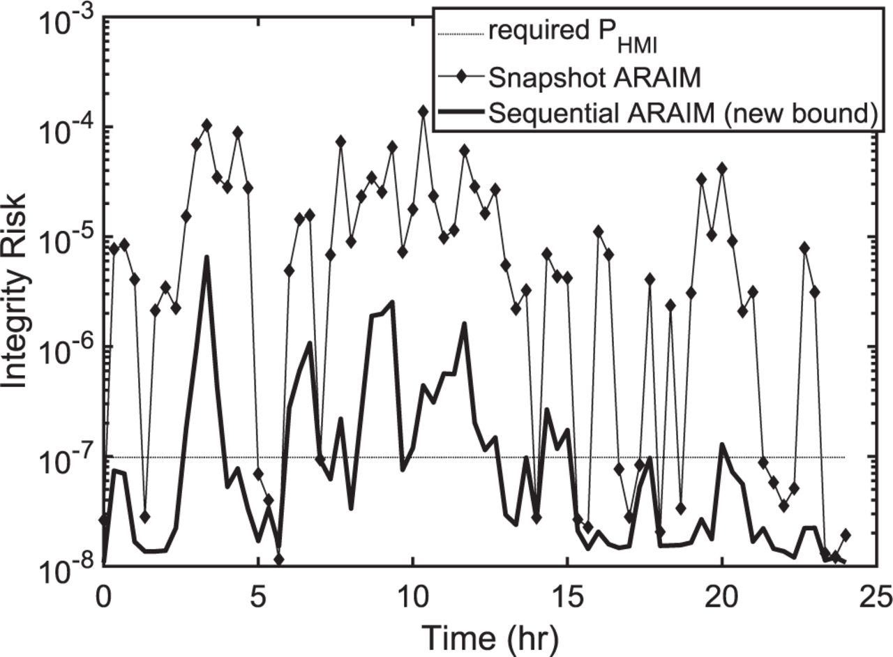
In Figure 5, the integrity risk is evaluated using sequential MHSS (Working Group C - ARAIM Technical Subgroup, 2016; Joerger & Pervan, 2020) over 24 hours, at an example Blacksburg, VA, location (37.2◦ N, −80.4◦ E), assuming dual-frequency measurements from GPS and Galileo. In this figure, in order to accentuate differences between implementations, we use a vertical alert limit of 10 m (instead of 35 m) and a prior probability of constellation faults of 10−8.

Integrity risk bound for snapshot versus sequential ARAIM with the non-stationary GM model. Bounds are computed using depleted constellations, 𝑃const = 10−8 and 𝓁 = 10 m
Figure 5 shows the significant integrity risk reduction obtained using sequential ARAIM (thick black curve) as compared to snapshot ARAIM (thin black curve with diamond markers). The fraction of time where the integrity risk curves are below the horizontal dotted line is the availability. In this case, availability is 60% for sequential ARAIM compared to 26% for snapshot ARAIM. The main conclusion from Figure 5 is not only that sequential ARAIM outperforms snapshot ARAIM as in Joerger and Pervan (2020), but also that we are still able to achieve substantial availability improvement even after accounting for our lack of knowledge in 𝜏𝜌, 𝜏𝜙 and 𝜏𝑇.
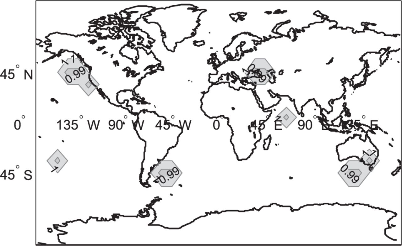
Figures 6 and 7 display global availability maps for a 10◦ ×10◦ latitude-longitude grid of locations, for satellite geometries simulated at regular 10-minute intervals over a 24-hour period. Availability is computed at each location as the fraction of time where the integrity risk bound is lower than the 10−7 requirement. The larger presence of white areas in Figure 7 compared to Figure 6 clearly indicates that snapshot ARAIM is outperformed by sequential ARAIM, even after accounting for measurement error time correlation uncertainty. The worldwide availability metric given in the figure captions is the weighted coverage of 99.5% availability. Coverage is defined as the percentage of grid point locations exceeding 99.5% availability. The coverage computation is weighted at each location by the cosine of the location’s latitude, because grid point locations near the equator represent larger areas than near the poles.

Availability map for snapshot ARAIM using depleted constellations, 𝑃const = 10−4,𝓁 = 35 m (coverage of 99.5% availability is 84.6%)

Availability map for sequential ARAIM with the non-stationary GM model using depleted constellations, 𝑃const = 10−4,𝓁 = 35 m (coverage of 99.5% availability is 97.8%)
Table 2 lists worldwide coverage of 99.5% availability, and of 95% availability (given in parentheses). It shows that the coverage of 99.5% availability increases from 84.6% for snapshot ARAIM to 97.8% for sequential ARAIM with the new non-stationary GM model, a 13% improvement for the case considered here. It is also worth pointing out that in Langel et al. (2019), we showed that if we knew 𝜏 = 𝜏max, 99.5% availability coverage for sequential ARAIM would be 99.5%. Thus, we sacrifice 1.7% of availability coverage due to time correlation uncertainty. These results would further improve with better knowledge of the measurement error sources, that is, if the difference between 𝜏max and 𝜏min could be reduced.
Coverage of 99.5% availability and coverage of 95% availability (in parentheses)
7 CONCLUSIONS
A new model for GM noise was developed that produces a KF covariance matrix that overbounds the estimate error distribution when the GM variances and time constants are uncertain. We proved that our model is applicable to both sampled-data and discrete-time systems, and demonstrated its performance for a one-dimensional estimation problem. For an aircraft navigation application using sequential ARAIM with our new model, it was shown that under specific circumstances, a larger than 10% improvement in 99.5% availability coverage is achievable compared to conventional snapshot ARAIM.
Future work will apply the results of this paper to other filtering applications like GNSS/INS integrated navigation. Research is also underway extending the ideas presented in the paper beyond first-order Gauss-Markov noise, with the goal of developing practical overbounding methods that do not rely on precise mathematical knowledge of the underlying time correlation.
HOW TO CITE THIS ARTICLE
Langel S, García Crespillo O, Joerger M. Overbounding the effect of uncertain Gauss-Markov noise in Kalman filtering. NAVIGATION. 2021;68(2):259–276. https://doi.org/10.1002/navi.419
ACKNOWLEDGMENTS
We would like to thank Dr. Juan Blanch of Stanford University for his comments and suggestions. His review was instrumental in ensuring that the technical development of the paper was conveyed as clearly as possible.
APPENDIX A: TRUE COVARIANCE MATRIX
This appendix derives the true estimate error covariance matrix for a state-augmented KF when there are uncertain parameters in the augmented state dynamic models. With  , the transition matrix in Equation (4) can be written as
 A1
A1
Then the dynamic model  in Equation (5) becomes
  . Noting that the KF estimate vector propagates as
  , the estimate error vector
  satisfies the differential equation
 A2
A2
Defining Δ𝐅𝑇 = [𝟎 Δ𝐋𝑇] and incorporating the dynamic model for the Gauss-Markov states results in the following propagation equation
 A3
A3
The estimate vector after the measurement update is  . It is straightforward to show that the estimate error vector is 𝜺𝑘|𝑘 = (𝐈− 𝐊𝑘𝐇𝑘)𝜺𝑘|𝑘−1 −𝐊𝑘𝐃𝑘𝒓𝑘. When combined with 𝒂𝑘 = 𝒂𝑘, the update equation is
 A4
A4
The covariance matrix 𝐏 = 𝐸[𝒆𝒆𝑇] propagates between measurements according to Simon (2006)
 A5
A5
where
 A6
A6
During a measurement update, the covariance matrix is updated through
 A7
A7
Equations (A5) and (A7) are identical to Equations (10) and (11) stated in Section 4.
APPENDIX B: INITIAL VARIANCE BOUND
This appendix derives the minimum allowable initial variance for the process in Equation (21). The derivation is based on the requirement that 𝚫(0) ≥ 0 and 𝚺𝑥𝑎(0) = 𝟎. If no prior information exists to initialize 𝒂 (the case considered here), the initial estimate for the augmented states is  . We also assume that
  and â0 are initially uncorrelated, so that
  .
.
This leads to the following expected values
 B8
B8
where we have used the fact that because â0 = 0,  ,
,  and
and  are all equal to 𝟎. Using these relations, the true initial covariance matrix of
  is
is
 B9
B9
The requirement 𝚺𝑥𝑎 = 𝟎 implies that
 B10
B10
The goal is to determine 𝚺𝑎,0 so that 𝚺(0) ≥ 𝐏(0). Subtracting 𝐏(0) from 𝚺(0) results in
 B11
B11
Using Schur complements (Gallier, 2019), 𝚺(0) ≥ 𝐏(0) if and only if
 B12
B12
It is assumed that 𝚺𝜉,0 can be determined so that (𝚺𝜉,0 − 𝐏𝜉,0) ≥ 0. Then it suffices to show that
 B13
B13
All matrices in Equation (B13) are diagonal. Denoting an arbitrary diagonal element of 𝚺𝑎,0,  and 𝐏𝑎,0 as
  ,
,  and 𝜎2, respectively, we can therefore consider the scalar condition
 B14
B14
It can be shown from Equation (20) that
 B15
B15
Substituting this result into Equation (B14) and simplifying yields
 B16
B16
With  and 𝜏 ∈ [𝜏min,𝜏max], the initial variance
  must satisfy the inequality
 B17
B17
APPENDIX C: DISCRETE-TIME COVARIANCE ERROR MATRIX
This appendix derives propagation equations for the covariance error matrix Δ associated with the discrete-time system
 C18
C18
where  and 𝒂𝑘 is a vector of first-order GMPs with unknown but bounded time constants. We assume
  and
and  can be spec-ified, and that
  is estimated with a KF that models uncertain GMPs using Equation (28), restated below
 C19
C19
With 𝜙 = 𝑒−Δ𝑡∕𝜏 and  , a discrete-time GMP is governed by the difference equation Rogers (2003) 𝑎𝑘+ 1 = 𝜙𝑎𝑘 +𝛾𝑤𝑘, such that 𝑤𝑘 ∼ WGN(0, 1). Therefore,
 C20
C20
For the process in Equation (C19), let us also define  and
and  so that
  is 𝐋𝑘 populated with
  and
and  is 𝐔𝑘 populated with
  . After defining
 C21
C21
the KF covariance matrix propagates according to Gelb et al. (1974)
 C22a
C22a
 C22b
C22b
where 𝐊𝑘 is the Kalman gain matrix and 𝚺𝑎,0 is a diagonal matrix populated with the  ’s from Equation (C19).
Following the same approach as in Section 4, it can be shown that the true covariance matrix propagates as
 C23a
C23a
 C23b
C23b
 C23c
C23c
such that  ,
,  and 𝐐𝑥,𝑘 has the same form as
  , except that
  and
and  are replaced with 𝐍𝑘 and 𝐔𝑘. A comparison between the KF and true covariance matrices is made using the same approach as in Section 5. That is, by specifying a propagation structure for the larger covariance matrix 𝚺 that facilitates forming the error matrix 𝚫𝑘|𝑘 = 𝚺𝑘|𝑘 −𝐏𝑘|𝑘. To this aim, we define propagation equations for 𝚺𝑘|𝑘 as
 C24a
C24a
 C24b
C24b
 C24c
C24c
where  is defined in Section 5.2 and
  is diagonal with 𝑖th diagonal element
  . The reader should be aware that these are not the only options for
  and
and  . Other matrices could be specified. We will focus on the particular realizations above because they are a logical choice and facilitate subsequent analysis.
The structure in Equations (C24b) and (C24c) ensures that 1) Equations (C22a) and (C22b) remain intact, 2) 𝚺0|0 ≥ 𝐏0|0, which was shown in Section 5.2, and 3) the lower right block of 𝚺𝑘|𝑘 is time-invariant and always equal to its initial value  . The next step is to form the differences 𝚺𝑘+ 1|𝑘 −𝐏𝑘+ 1|𝑘 and 𝚺𝑘|𝑘 −𝐏𝑘|𝑘 to define propagation equations for the covariance error matrix 𝚫. However, Equation (C24b) is not ideal because the matrix bracketing 𝚺𝑘|𝑘 on the right-hand side does not match the matrix bracketing 𝐏𝑘|𝑘 in Equation (C23b). In response, let us rewrite Equation (C24b) as
 C25
C25
where we utilize the fact that 𝚺 is a block diagonal matrix and that the lower right block is time invariant. Now we can subtract Equations (C23b) and (C23c) from Equations (C24b) and (C24c), resulting in the covariance error propagation equations
 C26
C26
 C27
C27
APPENDIX D: PROOF OF POSITIVE SEMI-DEFINITENESS
This appendix shows that the following matrix
 D28
D28
is positive semi-definite. Recalling that  and
and  , and using the definition for
  given in Equation (C21), 𝐖 can be written in the 3×3 block form
 D29
D29
where we have used the fact that 𝐐𝑘 has the same structure as  with
with  ,
,  replaced by 𝐍𝑘 and 𝐔𝑘.
Making the definitions
 D30a
D30a
 D30b
D30b
allows 𝐖 to be written as  . To prove that 𝐖 ≥ 0, we use the fact that with 𝐙 > 0 and invertible, 𝐖 ≥ 0 if and only if (Gallier, 2019)
 D31
D31
To show that 𝐙 > 0 and invertible, first note from Appendix C that  is a diagonal matrix with 𝑖th diagonal element
 D32
D32
Since 0 ≤ 𝜙𝑖 ≤ 1 and  . Thus, the necessary conditions that 𝐙 > 0 and invertible are satisfied.
Substituting Equations (D30a) and (D30b) into Equation (D31) results in
 D33
D33
One way to prove that 𝐒 ≥ 0 is to show that  and 𝚲 are both positive semi-definite. Since we assumed that
  , clearly
  . It is more difficult to assess whether 𝚲 ≥ 0. To proceed, first notice that 𝚲 is a diagonal matrix because it is a linear combination of products of diagonal matrices. Thus, we can prove that 𝚲 ≥ 0 by showing that the diagonal elements are always nonnegative.
D.1 Defining an arbitrary diagonal element of Λ
This subsection develops an expression for an arbitrary diagonal element of 𝚲. From Appendices B and C, the 𝑖th diagonal elements of each matrix in Equation (D33) are
 D34
D34
Substituting the expressions from Equation (D34) into Equation (D33), the 𝑖th diagonal element of 𝚲 is
 D35
D35
As  approaches
  gets smaller. Thus, we will focus on proving that 𝜆𝑖 ≥ 0 for the limiting case when
  . From this point forward, the 𝑖 index will be dropped to simplify notation. Let 𝑟 = 𝜏max∕𝜏min and 𝛽 = 𝜎2 𝜏max∕(𝜏 − 𝜏max). Then Equation (D34) shows that
  can be written as 𝜎2 = −2𝛽, and Equation (D35) simplifies to
 D36
D36
Defining the expression inside the square brackets in Equation (36) as −𝜔, we obtain the final form for 𝜆 used in this appendix
 D37
D37
D.2 Monotonicity of 𝜆
We will now show that 𝜆 is a monotonically increasing function of Δ𝑡 for any 𝜏, 𝜏min and 𝜏max satisfying 𝜏 ∈ [𝜏min,𝜏max] and 𝜏min ≤ 𝜏max. With this fact established, the range of 𝜆(Δ𝑡) is entirely defined by its values at Δ𝑡 = 0 and Δ𝑡 = ∞. The proof is based on the fact that a differentiable function is monotonically increasing if its derivative is nonnegative at every point in the function’s domain (Bermant, 1963). It is safe to use this criteria for monotonicity because 𝜆(Δ𝑡) is continuous and therefore differentiable.
From Equation (D37), we have the following derivatives
 D38
D38
which, after simplification, lead to the following expression for 𝑑𝜆∕𝑑Δ𝑡
 D39
D39
where 𝛾 = 𝜎2 +2𝛽 = 𝜎2(𝜏 + 𝜏max)∕(𝜏 − 𝜏max). It will be useful to define the quantity in square brackets as
 D40
D40
so that 𝑑𝜆∕𝑑Δ𝑡 = −(2𝛾𝜙∕𝜏)𝜓.
The factor −(2𝛾𝜙∕𝜏) is nonnegative, which follows from the fact that 𝛾 ≤ 0. Therefore, 𝑑𝜆∕𝑑Δ𝑡 will be nonnegative as long as 𝜓 ≥ 0. We can prove that 𝜓 is nonnegative by examining its behavior as a function of Δ𝑡.Agiven value Δ𝑡∗ uniquely determines the quantities  ,
,  ,
,  and 𝜔∗ that, when substituted into Equation (D40), produce the value 𝜓∗. In addition to giving us 𝜓∗, Equation (D40) also tells us that 𝜔∗ must be a root of the equation
  . A necessary condition for the quadratic equation to have at least one real root is that the discriminant
  is greater than or equal to zero (Manfrino et al., 2015), that is, if
 D41
D41
From the definitions in Equation (D40), notice that
 D42
D42
The term in brackets is always less than or equal to zero, which can be shown by considering the inequality
 D43
D43
Substituting the definitions for 𝛽, 𝑟 and 𝛾 into Equation (D43) results in the new inequality
 D44
D44
Equation (D44) can also be written as
 D45
D45
As a function of 𝜏, the left-hand side of Equatiion (D45) is a parabola that starts at zero when 𝜏 = 𝜏min, rises to its maximum value (𝜏max −𝜏min)2∕4 when 𝜏 = (𝜏min + 𝜏max)∕2, and then falls back to zero when 𝜏 = 𝜏max. Thus, the inequality in Equation (D45) is always true. Tracing this result back to Equation (D42), we can conclude that
 D46
D46
Given that Equation (D46) is valid for any 𝜏, 𝜏min,𝜏max and Δ𝑡, we can conclude from Equation (D41) that 𝜓∗ ≥ 0. Since Δ𝑡∗ is arbitrary, it must be that 𝜓 is nonnegative for all values of 𝜏, 𝜏min,𝜏max and Δ𝑡. This completes the proof that 𝑑𝜆∕𝑑Δ𝑡 ≥ 0 and therefore that 𝜆 is a monotonically increasing function of Δ𝑡.
D.3 Establishing the range of 𝜆
Since 𝜆 is a monotonically increasing function of Δ𝑡, the range of 𝜆 is entirely defined by its value at Δ𝑡 = 0 and Δ𝑡 = ∞. Substituting these values for Δ𝑡 into Equation (D37) leads to the conclusion that
 D47
D47
The sign of the right endpoint is dictated by the sign of the quantity 𝜏−2𝜏min +𝜏max. The minimum value of this quantity is 𝜏max −𝜏min when 𝜏 = 𝜏min. Since 𝜏min ≤ 𝜏max, the right endpoint is greater than or equal to zero.
We have therefore established that 𝜆 ≥ 0 for all admissible values of 𝜎2,𝜏,𝜏min,𝜏max and Δ𝑡. This completes the proof that the matrix in Equation (D28) is positive semidefinite.
Footnotes
Disclosure
The author’s affiliation with The MITRE Corporation is provided for identification purposes only and is not intended to convey or imply MITRE’s concurrence with, or support for, the positions, opinions, or viewpoints expressed by the author.
- Received January 14, 2020.
- Revision received July 22, 2020.
- Copyright © 2021 Institute of Navigation
This is an open access article under the terms of the Creative Commons Attribution License, which permits use, distribution and reproduction in any medium, provided the original work is properly cited.


Jump to section
- Article
- Abstract
- SUMMARY OF MAIN RESULT
- 1 INTRODUCTION
- 2 PROBLEM SETUP
- 3 MOTIVATIONAL EXAMPLE
- 4 TRUE COVARIANCE MATRIX
- 5 MODELING UNCERTAIN GM NOISE
- 6 APPLICATION TO SEQUENTIAL ARAIM PERFORMANCE ANALYSIS
- 7 CONCLUSIONS
- HOW TO CITE THIS ARTICLE
- ACKNOWLEDGMENTS
- APPENDIX A: TRUE COVARIANCE MATRIX
- APPENDIX B: INITIAL VARIANCE BOUND
- APPENDIX C: DISCRETE-TIME COVARIANCE ERROR MATRIX
- APPENDIX D: PROOF OF POSITIVE SEMI-DEFINITENESS
- Footnotes
- REFERENCES
- Figures & Data
- Supplemental
- References
- Info & Metrics
Related Articles
Cited By...
- No citing articles found.