

Abstract
The GNSS performance is significantly degraded in urban canyons because of the signal interferences caused by buildings. Besides the multipath and nonline-of-sight (NLOS) receptions, the diffraction effect frequently occurs in urban canyons, which will severely attenuate the signal strength when the satellite line-of-sight (LOS) transmitting path is close to the building edge. It is essential to evaluate the performance of current diffraction models for GNSS before applying mitigation. The detailed steps of applying the knife-edge model and the uniform geometrical theory of diffraction (UTD) model on GNSS are given, including the 𝐶∕𝑁0 and pseudorange simulation of the diffracted signal. The performances of both models are assessed using real data from two typical urban scenarios. The result shows the UTD can adequately model the GNSS diffraction effect even in a complicated urban area. Compared with the knife-edge model, the UTD achieves better modeling accuracy, whereas it requires higher computational loads.
1 INTRODUCTION
Global Navigation Satellite System (GNSS) has been used in various applications, including autonomous driving (Hussain & Zeadally, 2019), portable device localization (Humphreys et al., 2016), and location-based services (LBSs) (Chen et al., 2017). As the only sensor directly providing the absolute positioning solutions, the GNSS plays an essential role in navigation. By using the precise point positioning (PPP) (Zumberge et al., 1997) or the real-time kinematic (RTK) (Langley, 1998) technique, the standalone GNSS positioning accuracy can be enhanced to centimeter level, which fulfills the precision requirements of most position-related applications. However, the performance of GNSS is strictly relying on the operating environment. The surrounding objects could introduce interferences with the GNSS signal, which significantly degrade the positioning accuracy and reliability, especially in urban canyons.
GNSS signals can be easily blocked or reflected with extra delays by buildings in an urban area. By receiving both the direct and the reflected signal, or even worst, the reflected signal only, a severe error is introduced in the GNSS pseudorange measurement, namely the multipath effect or the non-line-of-sight (NLOS) reception (Groves, 2013), respectively. Those degraded measurements could lead to enormous positioning errors, possibly exceeding 50 meters (Hsu, 2018). Various techniques have been developed to mitigate the positioning error from reflections, such as the receiver autonomous integrity monitoring (RAIM) (Parkinson & Axelrad, 1988; Pesonen, 2011) and the optimal solution searching process (Ziedan, 2018). On the other hand, the GNSS measurement can also be interfered when the line-of-sight (LOS) signal is close to the building edge, namely the diffraction effect (Bradbury, 2007). The diffraction effect occurs in a limited region adjacent to the building edge and only introduces a decimetre-level delay in pseudorange (McGraw, Groves, & Ashman, 2019). However, the diffraction can significantly attenuate the GNSS signal strength and degrade the overall positioning performance, especially in the dense urban area as illustrated in Figure 1, where the satellite visibility is already degraded and many of the satellites are close to building edges. The rapid fluctuating phase and strongly attenuated amplitude of the diffracted signal may also introduce cycle slips (Breitsch et al., 2020).

The GNSS measurement availability and 𝐶∕𝑁0 in a typical urban canyon in Hong Kong. The purple curves denote the building boundaries. The color denotes the 𝐶∕𝑁0. The data is collected using a low-cost commercial GNSS receiver
For conventional GNSS positioning approaches, the carrier-to-noise ratio (𝐶∕𝑁0) is used to indicate the measurements’ quality and determine the weighting of measurements (Hartinger & Brunner, 1999; Langley, 1997). However, the diffracted signal could also have an attenuated 𝐶∕𝑁0 close to the multipath signal or NLOS reception, even though the corresponding pseudorange error is small. Hence, among the limited measurements in urban canyons, most of them are assigned with similar low weights, which degrades the performance of weighted least square (WLS) positioning. Recently, the 3D mapping aided (3DMA) GNSS techniques have been developed to improve the positioning accuracy in urban areas. One of the widely applied 3DMA GNSS techniques is shadow matching (Wang, Groves, & Ziebart, 2015; Zhang et al., 2020). It determines the user’s position by matching the satellite visibility between the estimation based on measurement 𝐶∕𝑁0 and the prediction from the 3D building model. Unfortunately, the diffracted signal always has a 𝐶∕𝑁0 between that from a typical LOS and NLOS, introducing a fuzzy region during the classification of the satellite visibility (Wang, Groves, & Ziebart, 2013). The 3DMA GNSS techniques are further improved by matching not only the satellite visibility but also the pseudorange measurement, such as the likelihood-based ranging (LBR) (Groves et al., 2020) and the ray-tracing (Hsu, Gu, & Kamijo, 2016; Suzuki & Kubo, 2013). However, the 𝐶∕𝑁0 is still employed as an essential parameter for pseudorange error classification or modeling, which can be influenced by the diffraction. Therefore, the diffraction is still an inescapable interference for positioning in urban canyons.
For mitigating the interference from diffraction, a straight-forward approach is to distinguish it from other effects and apply unique treatments. The availability of the GNSS diffraction is closely related to the geometrical relationship between the satellite, receiver, and obstacles, more specifically, the blockage of the Fresnel zone for the GNSS signal (Bradbury, 2008; Hristov, 2000). The obstruction of the Fresnel zone can be employed as the condition to exclude those potential diffracted signals (Zimmermann et al., 2019). There is still no accurate criteria to determine whether the measurement quality will be degraded by the diffraction effect, since it also depends on the antenna specification (Walker & Kubik, 1996). An alternative approach is to recognize the diffracted signal by its 𝐶∕𝑁0 from physical modeling. Based on the Huygens-Fresnel principle, the diffraction of the electric field power can be simplified and modeled with the knife-edge model (Icking, Kersten, Schön, 2020; Orfanidis, 2002). However, the spatial integral of this model becomes complicated for a dense urban scenario with multiple irregular distributed buildings. Similar to the reflection effect evaluated by the GNSS reflectometry (GNSS-R) (Jia & Pei, 2018; Zavorotny & Voronovich, 2000), the diffraction effect can be modeled as the coefficient with respect to the incident field based on the geometrical characteristics, namely the geometrical theory of diffraction (GTD) (Keller, 1962). The GTD is then extended as the uniform geometrical theory of diffraction (UTD) in order to be valid for the transition region adjacent to the shadow boundary (Kouyoumjian & Pathak, 1974). The UTD can obtain an evaluation of diffraction similar to the integration-based method, through intuitive geometrical relationships (McNamara, Pistorius, & Malherbe, 1990). The UTD is also integrated with 3DMA GNSS to simulate the diffraction effect, aiding the positioning in urban areas (Suzuki & Kubo, 2012). Besides, there is an urgent need for a realistic urban GNSS simulator considering diffraction (Kbayer & Sahmoudi, 2018), especially for those urban GNSS positioning studies hard to be verified by real experiments, such as the GNSS-based collaborative positioning (Zhang et al., 2020).
Although there exists various studies employing the UTD and the 3D building model to evaluate the diffraction effect (Fan & Ding, 2006; Nicolás et al., 2012; Panicciari, Soliman, & Moura, 2017; Suzuki & Kubo, 2012), neither of them presents the detailed procedure and interpretation, especially for practical GNSS positioning applications. Besides, many of the studies treat the GNSS diffractions the same way as reflections when applying interference mitigation techniques (Bisnath & Langley, 2001; Realini & Reguzzoni, 2013; Zhang et al., 2020) without a specific consideration about its influence and characteristics. In this study, we will focus on simulating the GNSS diffraction through the knife-edge model and the UTD approach. Then, the resultant diffraction coefficient from both approaches is employed to simulate the diffraction effects on the GNSS 𝐶∕𝑁0 and pseudorange. Finally, the simulation performance is validated and analyzed with real experimental GNSS measurements in an urban area of Hong Kong. The contribution of this study is twofold: 1) The GNSS 𝐶∕𝑁0 and pseudorange measurements under diffraction are simulated with detailed procedures and interpretations; 2) The diffraction simulation performance is assessed with real consumer-grade GNSS measurements collected in an urban environment, including the discussion on the model accuracy, computation load, and potential contributions.
It is worth mentioning that the performance of the GNSS diffraction modeling by the UTD has been preliminarily investigated by (Nicolás et al., 2012). In this study, the 𝐶∕𝑁0 of the GNSS signal is simulated by applying the UTD model with the ray-tracing and channel-modeling results. The simulation results show great consistency with the real measurements, revealing the feasibility of precisely modeling the GNSS diffraction effects. Inspired by this study, comprehensive diffraction modeling performance assessment and analysis for the urban scenario are conducted in this paper. Although both studies employ the same fundamental UTD model (Kouyoumjian & Pathak, 1974), several extensions are made in this study. First, instead of applying channel modeling, an open-sky 𝐶∕𝑁0 regression model is employed for the 𝐶∕𝑁0 simulation of the diffracted signal, which reduces the modeling complexity for the applications only using measurement-level GNSS data. Second, a comprehensive analysis of the diffraction modeling is presented, including the effect on pseudorange, the relationship with building accuracy, and a comparison with the knife-edge model on accuracy and computational cost. Finally, our diffraction modeling performance assessment focuses on the low-cost receiver in a dense urban scenario, where more unexpected interferences other than the diffraction possibly exist. Therefore, this study can be regarded as a detailed and comprehensive extension of the aforementioned preliminary study to the dense urban scenarios.
The remainder of this paper is structured as follows. Section 2 introduces the diffraction modeling of a GNSS signal based on the knife-edge model. Section 3 gives a brief introduction to diffraction modeling using the UTD. The detailed procedures for practical GNSS diffraction simulation are given in Section 4, including the simulation of GNSS 𝐶∕𝑁0 and pseudorange measurement. The experimental validation of GNSS diffraction simulation is demonstrated in Section 5. Finally, the conclusion is drawn in Section 6.
2 KNIFE-EDGE DIFFRACTION MODEL
For a regular case where the GNSS measurement LOS vector (direct path from the satellite to the receiver) is perpendicular to the building edge, the corresponding diffraction can be simplified to an electric field attenuated by a knife-like edge in 2-dimension (2D). In this section, the Huygens-Fresnel principle on the knife-edge diffraction is briefly introduced, which describes diffraction as a total effect of all unobstructed secondary wavelets in space. Then, the Fresnel integral is employed to evaluate the diffraction attenuation by this total effect quantitatively.
2.1 Huygens-Fresnel principle
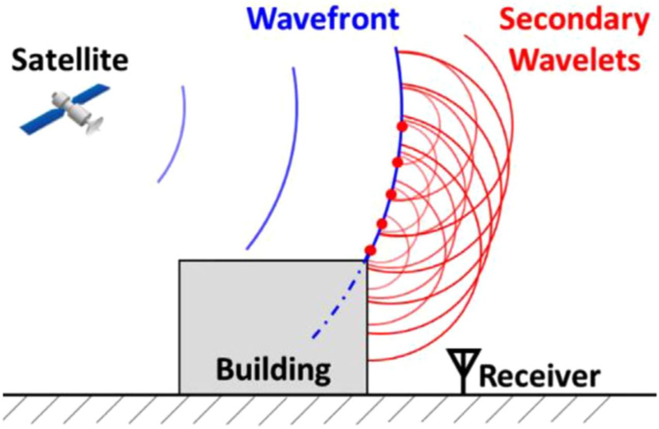
The fundamental law for the knife-edge model is the Huygens-Fresnel principle (Hristov, 2000). As shown in Figure 2, the Huygens-Fresnel principle states that each infinitesimal point of a wavefront emits a spherical wavelet. The secondary wavelets interfere with each other and jointly form a new wavefront. When part of the wavefront is obstructed, the receiver can only receive the total effect of those secondary wavelets emitted from the unobstructed part of the wavefront. Hence, the diffraction is the incompleteness of the collective effect from the secondary wavelets on a partially blocked wavefront, noted that the phase difference of each secondary wavelet on a reference point (e.g., the receiver) will introduce constructive or destructive interference in between. Hence, the geometrical relationship between the obstacle and the reference point determines the corresponding total constructive/destructive effect; in other words, the field attenuation.

The demonstration of the Huygens-Fresnel principle for GNSS diffraction
2.2 Evaluation with Fresnel integral
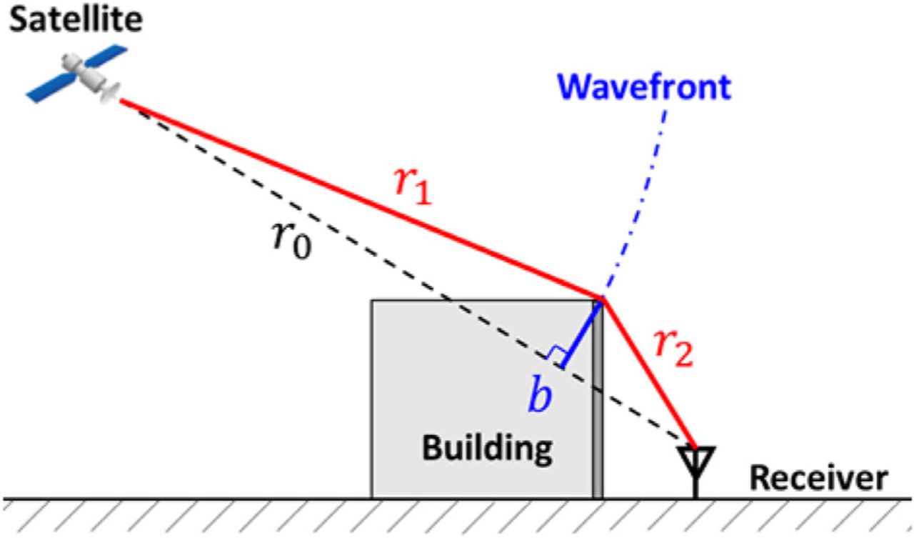
The GNSS diffraction effect for the receiver in Figure 2 can be represented as the superposition of the contribution from all secondary wavelets. Since the satellite is far away from the user compared to the building, the wavefront crossing the building edge and emitting secondary wavelets can be approximated as a plane in Figure 3. By applying the spatial integral on the passing through the wavefront (Orfanidis, 2002), the unobstructed/diffracted field ratio, namely the diffraction coefficient, can be estimated as follows:
 1
1
 2
2

The GNSS diffraction evaluation based on the knife-edge model
where 𝐹(𝜐) denotes the Fresnel integral. Variable 𝜐 is determined by the signal wavelength 𝜆 and the geometrical parameter 𝑏, which relates to the satellite elevation angle, the elevation angle of the building edge and the building height (refer to Figure 3). By knowing the geometrical parameters, the corresponding diffraction coefficient can be derived and further used to evaluate the 𝐶∕𝑁0 of a diffracted signal.
3 UNIFORM GEOMETRICAL THEORY OF DIFFRACTION
The preceding diffraction modeling approach involves a spatial integral, which is complicated for the scenario with multiple irregularly distributed obstacles, such as the dense urban environment. Therefore, it is convenient to employ the UTD approach, which models the diffraction as a geometric-related local effect dominated by a single ray passing through the obstacle edge. In modern geometrical optics (GO), the free-space propagation model is derived to describe the electric field behavior during the propagation in a certain media without obstruction. The UTD then describes the diffraction by extending the free-space propagation model with a geometry-related coefficient due to obstruction.
3.1 Free-space propagation model
The UTD is built up based on the modern geometrical optics (GO), which extends the classical geometrical optics with Maxwell’s equations and the Luneberg-Kline expansion (McNamara et al., 1990). For the high-frequency field, such as GNSS signals, the property variation of the medium or the scatter obstacle is negligible over the scale of the wavelength. Then, the total effect of the field can be asymptotically represented by the local effect of a scatter. In GO, the free-space propagation of high-frequency electric field with spherical wavefront can be expressed by
 3
3
 4
4
where 𝐄(𝑠) denotes the electric field with a distance 𝑠 along the direct propagation path from a reference point. The term 𝐄(0) denotes the field on the reference point 𝑠 = 0, consisting of the field amplitude 𝐄𝑎𝑚𝑝(0) on the polarization direction and the reference phase component 𝑒−𝑗𝑘Ψ(0) with phase function Ψ(0). The term  is usually denoted as the spreading factor 𝐴(𝑠), representing the amplitude variation along with propagation. 𝛾1 and 𝛾2 are the principal radii of the wavefront curvature. For example, the plane wave has the radii 𝛾1,𝛾2 → ∞, reducing the propagation expression as 𝐄(𝑠) = 𝐄(0)𝑒−𝑗𝑘𝑠. The term 𝑒−𝑗𝑘𝑠 represents the phase shift with wavenumber 𝑘 during propagation. From this expression, we can evaluate the electric field on a specified location based on the knowledge of that field on a reference point.
3.2 3D Diffraction model
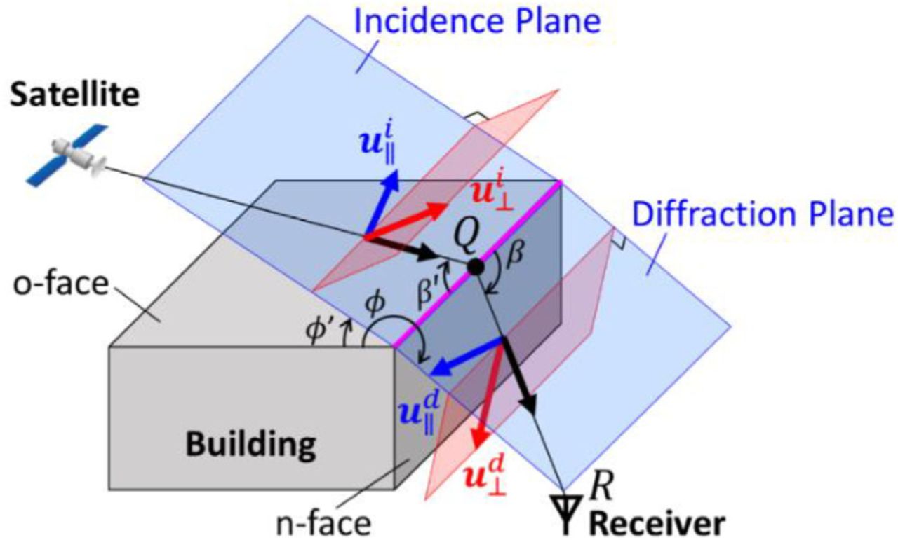
Following Fermat’s principle (Keller, 1962), the local effect of the GNSS diffraction shall be represented by the point achieving the shortest distance between the satellite and the receiver along the line of edge, denoted as the point of diffraction 𝑄 in Figure 4. Consequently, the angle 𝛽′ between the incident ray and edge is equal to the angle 𝛽 between the diffraction path and edge. Analogous to the reflection effect, the expression of the diffracted field from a perfectly conducting structure follows the GO free-space propagation model, but with the diffraction coefficient (Kouyoumjian & Pathak, 1974) 𝐷∥,⊥, as follows:
 5
5

The GNSS diffraction evaluation based on UTD (McNamara et al., 1990; Nicolás et al., 2012)
where  and
and  denote the two orthogonal components of the diffracted field along the unit vector
  and
and  on location 𝑅, parallel and perpendicular to the diffraction plane (the plane containing the diffracted ray and the obstacle edge), respectively. Here, the unit vectors of propagation direction, ∥, and ⊥ directions are following the right-hand rule. Similarly,
  and
and  denote the two orthogonal components of the incidence field on location 𝑄, parallel and perpendicular to the incidence plane (the plane containing the incidence ray and the obstacle edge), respectively. Here, we employ a decomposition coordinate the same as (McNamara et al., 1990), which may have a different definition on ∥ and ⊥ compared to some of the other studies. The decomposition of the incident field is aiming to account for the diffraction effect differently on the ∥ and ⊥ component. The connection between the incident and the diffracted field is described by Equation (5) with the diffraction coefficient 𝐷∥ and 𝐷⊥, which are given by (Kouyoumjian & Pathak, 1974) as follows:
 6
6
 7
7
 8
8
 9
9
 10
10
 11
11
where 𝐷1 and 𝐷2 are related to the diffraction effect when the o-face and the n-face of an obstacle are shadowed, while 𝐷3 and 𝐷4 are related to the diffraction effect when there also exist valid reflections from the n-face and the o-face of an obstacle to the location 𝑅. The variable 𝑇(𝑥) is a transition function (McNamara et al., 1990) which can be numerically calculated based on the geometrical parameters in Figure 4 and the wavenumber 𝑘. The term 𝑎±(𝜙 ± 𝜙′) = 2cos2{[2𝑛𝜋𝑁± −(𝜙±𝜙′)]∕2} is a geometry-related function (Kouyoumjian & Pathak, 1974), where 𝑁± is the integer most nearly satisfying 2𝑛𝜋𝑁± −(𝜙±𝜙′) = ±𝜋 based on the angle 𝜙′ from the o-face to the incidence plane and 𝜙 from the o-face to the diffraction plane.
For the case of GNSS signals, the diffraction always occurs in a scenario with typical geometrical features, which can simplify the preceding expressions. In practice, the level-of-detail-1 (LOD-1) building model (Groves, 2016) is employed during the diffraction modeling, where the building edges are simplified as straight lines. Hence, the diffracted field wavefront is cylindrically emitted from a line source field along the building edge, resulting in a spreading factor  . According to (McNamara et al., 1990), the parameter 𝑛 can be assigned with 1.5 representing a 90-degree diffracting wedge angle, because the LOD-1 building model is always vertically mounted on the ground and has a flat roof. Since the satellite is far away from the building and the receiver (𝑟1 ≫ 𝑟2), the incident field can be approximated as plane-wave incidence, making the distance parameter 𝐿 = 𝑟2sin2𝛽. Since it is hard to precisely describe the building material in the complex urban environment, the structures introducing diffractions are assumed to be perfectly conducting structures for simplification. In most cases, the GNSS receiver suffering diffraction is below the building roof and with a certain distance to the building. It is less likely to enter the zone occurring reflection and diffraction simultaneously for the same building, which reduces the diffraction coefficient as 𝐷∥,⊥ = 𝐷1 +𝐷2.
4 GNSS DIFFRACTION SIMULATIONS
The procedures of GNSS diffraction simulation are demonstrated in this section, including the 𝐶∕𝑁0 and the pseudorange simulation of the diffracted signal and the diffraction availability.
4.1 Overview
The GNSS diffraction simulation architecture is demonstrated as shown in Figure 5. The ephemeris provides the satellite position 𝐱𝑆𝑉 for a specific time. The 3D building model is commonly in the LOD-1, which is denoted by matrix 𝐗𝐵 containing all the corner locations of each building. Based on 𝐱𝑆𝑉, 𝐗𝐵, and the receiver location 𝐱𝑅, the geometrical parameters of the building introducing diffraction can be obtained through the ray-tracing technique. For the diffraction simulation based on the knife-edge model, the diffraction coefficient can be evaluated by the geometry-related parameters 𝑏 and 𝑟2. For the UTD approach, the location of the diffraction point on the building edge, which dominates the diffraction effect, needs to be obtained beforehand. After searching for the location satisfies the geometrical condition of diffraction by raytracing, the UTD employs the geometrical parameters of the diffraction point to obtain the diffraction coefficient of the field. Then, the modeled open-sky 𝐶∕𝑁0 and the diffraction coefficient from the knife-edge model or UTD are combined to simulate the 𝐶∕𝑁0 of the diffracted signal. Moreover, the diffraction effect on GNSS pseudorange can also be simulated after applying UTD. The distances between satellite, receiver, and the diffraction point are estimated during the ray-tracing. The GNSS diffracted pseudorange can be simulated by combining the systematic error 𝜀𝜌 from the pseudorange error model, which considers the atmospheric delay and satellite clock/orbit bias. During the pseudorange simulation, if the satellite LOS vector is unobstructed, there exists the influence of the direct field, besides the diffracted field on edge. The interference between the direct and the diffracted field on pseudorange needs to be estimated by the corresponding 𝐶∕𝑁0 and the multipath noise envelope. At this point, both the GNSS 𝐶∕𝑁0 and pseudorange measurements under diffraction are simulated through the flowchart.

The flowchart of the GNSS diffraction simulation
4.2 𝑪∕𝑵𝟎 of the diffraction signal
Both the knife-edge model and the UTD are derived based on the linear polarized electric field, whereas the GNSS signal is right-hand circularly polarized (RHCP). The circular polarized field of GNSS can be considered as the superposition of two orthogonal linear polarized fields with a quarter phase shift in between. Similar to GNSS-R (Jia & Pei, 2018), the overall diffraction is evaluated by combining the individual diffraction effect on each decomposed linear polarized field.
For the knife-edge model approach, the 𝐶∕𝑁0 of the diffracted signal is simulated based on the 2D model in Section 2.2, which simplifies the 3D case with the same cross sections. We first use ray-tracing to search for the building closest to the LOS vector of the satellite, which probably introduces diffraction. The corresponding building height and the elevation angle of the building edge on the satellite’s azimuth angle direction are employed to derive the geometrical parameters 𝑏 and 𝑟2 based on Algorithm 1. Then, the diffraction coefficient of a linear polarized field related to that building can be estimated by the knife-edge model with Equations (1) and (2) as shown in Figure 5. For the GNSS signal with RHCP, the corresponding diffraction coefficient can be derived as the averaged coefficient of its two orthogonally decomposed linear fields (Stutzman, 1993). Those decomposed fields have the same diffraction coefficient from the knife-edge model, which makes the averaged diffraction coefficient for the RHCP field also the same. Therefore, the 𝐷𝑘𝑛𝑖𝑓𝑒−𝑒𝑑𝑔𝑒 from Equations (1) and (2) can be directly employed to indicate the overall diffraction coefficient of the RHCP GNSS signal and used to simulate the 𝐶∕𝑁0 and pseudorange of the diffracted signal later.
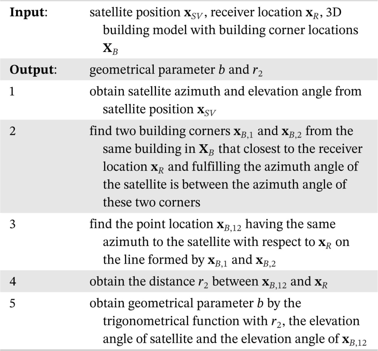
Ray-tracing for the knife edge model
For the UTD approach, unlike the knife-edge model, it approximates the diffraction as a local effect on a particular location along the building edge, namely the diffraction point. Hence, the location of the diffraction point needs to be obtained beforehand. Based on the satellite position, receiver position, and the 3D building model, the feasible diffraction point can be located via ray-tracing, searching the points satisfying that the angle between incidence and edge is equal to that between the diffraction path and edge. The detailed procedures of the diffraction point searching and the corresponding geometrical parameters calculation are demonstrated in Algorithm 2. The geometrical parameters of that diffraction point can then be used to estimate the diffraction coefficient related to that building edge for a linear polarized incident field by Equations (5)-(11). However, the preceding UTD is developed for the linear polarized fields, whereas the GNSS signal is normally transmitted using RHCP. Additional conversion is needed for the UTD to model the diffraction effect of the RHCP GNSS signal, noted the conversion between linear polarized and RHCP field here is different from the knife-edge model since the UTD approximates the diffraction as a local effect.
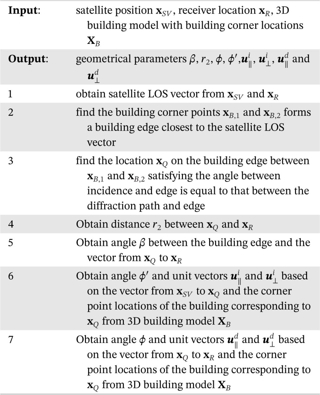
Ray-tracing for the UTD approach
In UTD, the GNSS signal experiences a transition on the building edge from the incident field to the diffracted field. As shown in Figure 4, the corresponding RHCP field can be orthogonally decomposed into two linear polarized fields, the soft diffraction component denoted by ∥, and the hard diffraction component denoted by ⊥. The decomposed fields behave differently during this transition according to the geometrical relationship to the edge. Knowing the GNSS field maintains RHCP during diffraction (Maqsood et al., 2013), the dyadic diffraction coefficient for the RHCP field can then be derived based on the dyadic diffraction coefficient for those linear fields (McNamara et al., 1990) and the circular polarization mechanism (Stutzman, 1993):
 12
12
where  and
and  denote the incident and the diffracted RHCP field, respectively. Variables
  ,
,  ,
,  , and
, and  are the unit vectors defined in Section 2.2, which are used to describe the transition behavior for each decomposed field during diffraction.
Unlike the knife-edge model naturally includes all the field interferences by the integral, the UTD approximates the phenomenon as a local effect. When the GNSS LOS signal is also unobstructed, the interference between the LOS and the diffracted field needs to be additionally considered. Therefore, by including the spreading factor and phase shift, the overall diffraction coefficient on the receiver location for different conditions are derived as follows:
 13
13
where 𝛿𝑟 is the extra distance of the diffracted path compared to the unobstructed path, 𝑟2 is the distance between the diffraction point and receiver. Here, the LOS field is simplified with the spreading factor of a plane wave, 𝐴(𝑠) = 1, since the satellite is very far from the receiver.
For the scenario with diffractions from multiple edges, such as the narrow gap between buildings in a dense urban area, the geometrical parameters of the corresponding diffracted field are obtained by repeating Algorithm 2 on those edges. After calculating the diffraction coefficient of each diffracted field, the overall diffraction coefficient is derived by the superposition of diffracted fields from all the related edges, as
 14
14
where 𝐷𝑅𝑅,𝑚, 𝐴𝑚, and Ψ𝑚 denote the diffraction coefficient, spreading factor, and phase shift distance from the reference field for the 𝑚𝑡ℎ edge, respectively. The variable Ψ0 denotes the phase shift distance between the LOS field and the reference field, which may not be the same in some cases. Then, the overall diffraction coefficient from UTD, 𝐷𝑈𝑇𝐷, can be used to simulate the 𝐶∕𝑁0 and pseudorange of the diffracted signal. For most practical cases, only the closest building edge dominating the diffraction effect needs to be considered, which reduces Equation (14) to Equation (13).
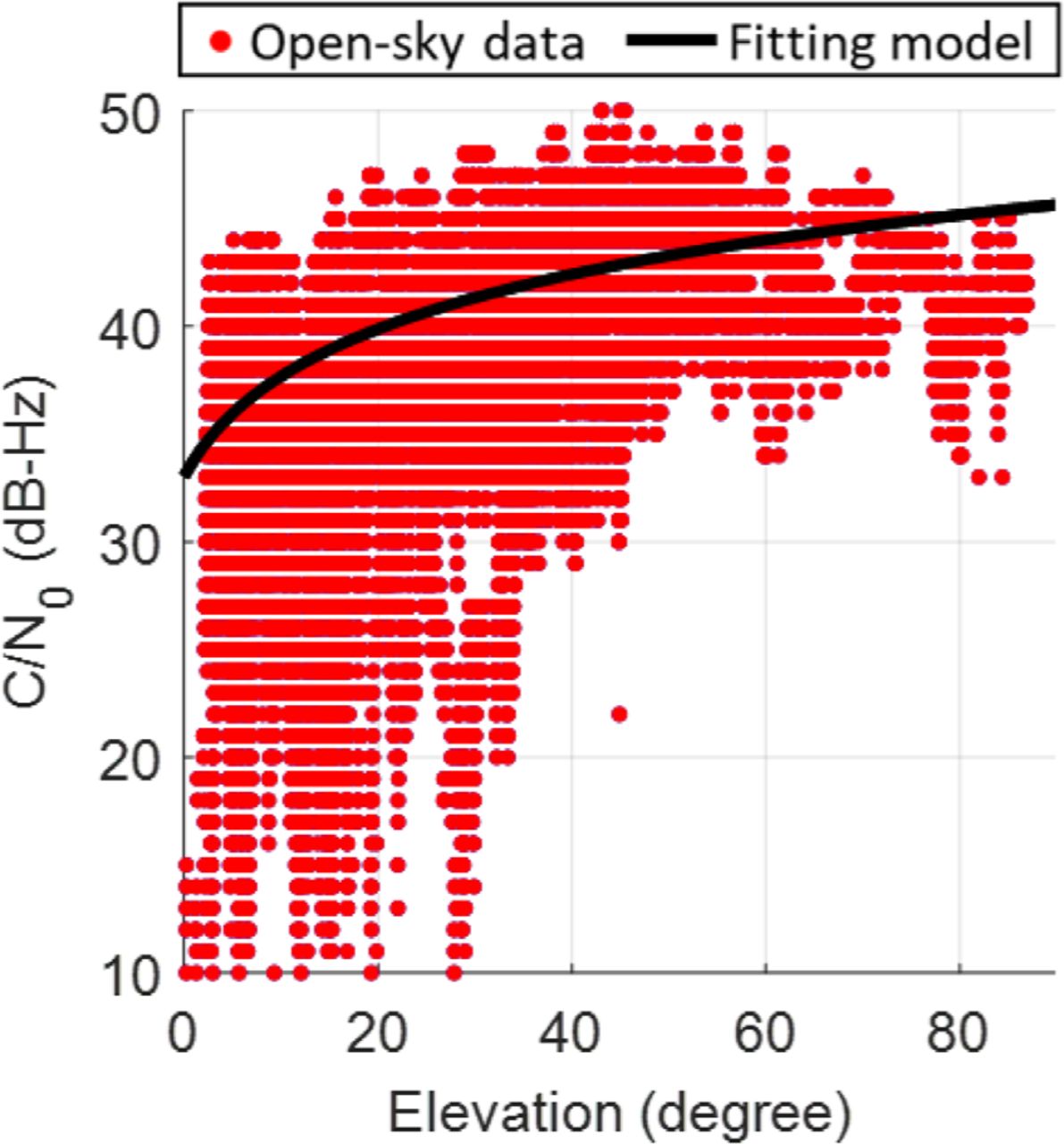
After obtaining the overall diffraction coefficient, the incident field strength is also required to simulate the diffracted field strength. However, it is hard to directly obtain the incident field, which relates to atmospheric interference or other effects. A practical approach is to employ an open-sky GNSS elevation-𝐶∕𝑁0 regression model from long period data (Suzuki & Kubo, 2012). In this study, the model is obtained through the first-order polynomial fitting on the four hours open-sky GNSS elevation angle and 𝐶∕𝑁0 (in the unit of Hz) data with respect to different satellite orbits. An example of the fitting model for the GPS satellite is shown in Figure 6. Then, the incident field strength of a specific satellite can be described by its unobstructed 𝐶∕𝑁0 from the model. Since the 𝐶∕𝑁0 relates to the signal power, the diffraction coefficient expressed in the power ratio is given by
 15
15

Example of the open-sky GNSS elevation-𝐶∕𝑁0 regression model for the GPS measurements
where 𝑃𝑑 and 𝑃𝑖 denote the diffracted and the incident field power, respectively. The term 𝐷𝑘𝑛𝑖𝑓𝑒−𝑒𝑑𝑔𝑒,𝑈𝑇𝐷 is the overall diffraction coefficient from the knife-edge model or UTD. Based on the formulation of signal-to-noise ratio (SNR) (Jia & Pei, 2018) and the conversion between SNR and 𝐶∕𝑁0 (Joseph, 2010), the 𝐶∕𝑁0 of a diffracted GNSS signal is derived as follows:
 16
16
where 𝐶∕𝑁0,𝑜𝑝𝑒𝑛 is the unobstructed 𝐶∕𝑁0 predicted by the open-sky model based on the satellite elevation angle. Here, the influence of the 𝐶∕𝑁0 from the diffraction delay is neglected, since this delay is negligible compared to the total traveling distance.
4.3 Diffracted pseudorange
The GNSS pseudorange is a ranging measurement based on the time-of-arrival (TOA) from satellite to receiver. During the UTD simulation, the distance 𝑟0 from satellite to receiver, 𝑟1 from satellite to diffraction point, and 𝑟2 from diffraction point to receiver can be obtained from the raytracing and used to simulate the GNSS ranging measurement on the dominating signal path. However, for the knife-edge model, the diffraction effect is modeled as a cumulating effect via integral. The ray-tracing there is only used to obtain the geometrical parameters of the integral area. Therefore, unlike the UTD approach, the diffraction effect on the pseudorange in the knife-edge model is not dominated by a single signal path, and it needs a complicated integration process that will not be simulated in this study. For the diffracted satellite being blocked by the buildings, namely NLOS diffraction, the signal delay due to diffraction can be evaluated by 𝑟0, 𝑟1, and 𝑟2, denoted as 𝜀𝑑 = 𝑟1 +𝑟2 −𝑟0. Then, the diffracted pseudorange can be simulated by combing the LOS distance 𝑟0, diffraction delay 𝜀𝑑, and the systematic error 𝜀𝜌, including the atmospheric delay and satellite clock/orbit bias from models (Kaplan & Hegarty, 2017). For the diffracted satellite not being blocked by buildings, namely LOS diffraction, the interference between the diffracted signal and the direct signal needs to be considered in addition. This interference can be modeled by the multipath noise envelope (Liu & Amin, 2009) based on the ranging delay 𝜀𝑑, the carrier-phase offset 𝛽 = −𝑘𝜀𝑑, and the 𝐶∕𝑁0 ratio between the diffracted and the direct signal, denoted as a function 𝜀𝑚𝑝(𝜀𝑑,𝐶∕𝑁0,𝑜𝑝𝑒𝑛,𝐶∕𝑁0,𝑑𝑖𝑓𝑓𝑟𝑎𝑐𝑡𝑖𝑜𝑛). In this study, we only consider the strongest two fields for the scenario with multiple fields. Since it is hard to know the time spacing between the early and late correlators for various low-cost receivers, the correlator spacing here is assumed to be 1 chip. Therefore, the diffracted pseudorange for LOS or NLOS condition is simulated by
 17
17
Compared to the LOS signal without diffraction, the pseudorange error due to NLOS diffraction and LOS diffraction is 𝜀𝑑 and 𝜀𝑚𝑝, respectively. Since the diffraction delay is usually in decimeter level (McGraw et al., 2019), the pseudorange error due to diffraction is generally negligible compared to the user-equivalent-range-error (UERE) 𝜎𝑈𝐸𝑅𝐸 ≈ 7𝑚 in practical cases (Kaplan & Hegarty, 2017).
4.4 Diffraction availability
Besides simulating the quantitative value of the 𝐶∕𝑁0 and pseudorange of the diffracted signal, the availability of these diffracted measurements is also required to be considered. When the satellite elevation angle is descending below the building edge introducing diffraction, the signal is increasingly attenuated, until it is too weak to be received by the receiver. The connection between signal availability and geometrical properties is related to the Fresnel zone of the signal.
From the Huygens-Fresnel principle (Figure 2), each point on the wavefront has a different distance to the receiver, introducing the phase difference between secondary wavelets. Compared to the secondary wavelet on the LOS vector, some of the secondary wavelets are constructive while others are destructive. The secondary wavelets with constructive or destructive interference are respectively located in certain regions, which are the Fresnel zones demonstrated in Figure 7. The boundary of each zone is defined by
 18
18

The demonstration of Fresnel zone blockage during diffraction
where 𝑁𝐹 is a positive integer number. 𝑟0 is the distance between satellite and receiver. The variable 𝑟𝑎 is the distance between a satellite and a wavefront, and 𝑟𝑏 is the distance from the secondary wavelet on that wavefront to the receiver. The secondary wavelet located in the 1st Zone (Figure 7) has an extra travelling distance below half of the wavelength compared to that on the LOS vector, which introduces constructive interference. Similarly, the secondary wavelet in the zones with odd integer 𝑁𝐹 is constructive with respect to the secondary wavelet on the LOS vector. In contrast, the secondary wavelet lies in the even numbered zones introduces destructive interference. The wave propagation can be regarded as a total effect of secondary wavelets from all these zones with constructive or destructive effects.
For the GNSS signal with a short wavelength, the constructive or destructive zones are narrowly spread in the space and rapidly canceling each other. The total effect can be represented by the first several zones (Hristov, 2000). Then, the field attenuation under diffraction is depending on the blockage of the first several zones, or more directly, the first zone with the highest constructive effect (Bradbury, 2008). As shown in Figure 7, the signal is less likely to be available for the receiver when most of the first zone is being blocked. A rule of thumb to determine the signal availability is by a threshold of 60% blockage (Bradbury, 2008). By checking the blockage ratio of the first Fresnel zone, the signal availability for the receiver can be predicted during the simulation. However, this prediction is only appropriate for the geodetic receiver. For the low-cost receiver with higher sensitivity, the measurement may still be available even though the 1st Fresnel zone is entirely blocked.
5 EXPERIMENTAL VALIDATIONS
5.1 Experiment setup
To evaluate the performance of the simulated GNSS 𝐶∕𝑁0 after diffraction using the knife-edge model and the UTD, two static experiments are conducted in the urban canyons in Hong Kong, as shown in Figure 8. The first experiment is located with one-side blockage by a single building. Here, the receptions of the blocked satellites are only due to diffractions since no valid reflection exists from other buildings (means no long- and middle-range reflections exist). The second experiment is located in a deep urban canyon surrounded by multiple buildings, where reflections and diffractions may occur simultaneously. A consumer-grade GNSS receiver ublox EVK-M8T with a patched antenna is used to record measurements on both sites. The GNSS antenna is placed on a flat surface for both scenarios, as shown in Figure 8, to mitigate the ground reflections. The receiver’s true location is obtained based on the landmarks on Google Earth, which the accuracy is within 1-2 meters based on our experience. The 3D building model for simulation is also extracted from Google Earth. From the skyplots of Figure 8, the 𝐶∕𝑁0 of the satellites moving across the building edge in both two tests are having significant attenuations, which are very likely due to diffractions. In the following sections, the measurements of these satellites are used to validate the diffraction simulation performance.

The surrounding environment and the diffracted satellite 𝐶∕𝑁0 in the skyplot during the validation experiments. The 𝐶∕𝑁0 is given by a low-cost commercial GNSS receiver
5.2 Validation on the one-side building scenario
For the diffracted signal from satellite G27 in the one-side building scenario, the comparison of 𝐶∕𝑁0 between real received measurement and the simulation from the knife-edge model or UTD are shown in Figure 9. The blockage ratio of the first Fresnel zone is also shown correspondingly, which is commonly used to evaluate the signal strength attenuation. The signal gets higher attenuation when the blockage ratio of the first Fresnel zone is increased. Here, the LOS vector of the satellite is nearly perpendicular to the building edge, which is ideal for the knife-edge model. The knife-edge model and UTD yield similar simulation results for the 𝐶∕𝑁0, which agree with the received measurements. In line with the prediction, the measurements 𝐶∕𝑁0 starts decreasing when the building edges enter the first Fresnel zone of the signal. Therefore, the measurement has already been attenuated before its LOS vector is blocked by the building; in other words, the LOS measurement close to the building edge could already be affected by diffraction. However, even though the first Fresnel zone has been completely blocked, the measurement is still available with very low 𝐶∕𝑁0. It is probably because the sensitivity of a low-cost receiver is much higher than that of the geodetic receiver (Bradbury, 2008, Walker & Kubik, 1996). A similar phenomenon is also observed in (Icking et al., 2020). Hence, for a low-cost receiver, the diffraction may still occur even when the satellite elevation angle is much lower than the building (see Section 5.6 for the details).

The diffraction simulation result for satellite G27 in the one-side building scenario, including: (a) comparison of the 𝐶∕𝑁0 from the knife-edge model or UTD simulation and real measurements; (b) the blockage ratio of the first Fresnel zone; (c) the elevation angles of the satellite and the elevation angles of the building edge in the azimuth direction of the satellite; and (d) the pseudorange error from simulated diffraction and real measurement
The pseudorange error from simulated diffraction is compared with that from the real measurement for G27 in Figure 9 (d). The pseudorange error from measurement is estimated using the double difference (DD) approach based on the measurement and the actual location of the receiver and a reference station (Xu et al., 2019). During the diffraction period between purple dash lines, the simulated pseudorange error is in decimeter level and negligible compared to 𝜎𝑈𝐸𝑅𝐸. Meanwhile, the DD-estimated pseudorange error from the real measurement is around 4 meters, which is the same as the period before the first Fresnel zone blockage starts. Noted that the DD approach is employed to eliminate the receiver/satellite clock errors during the pseudorange error estimation through a differential process with the measurement from a selected master satellite (usually with the highest elevation angle). However, the multipath error from the master satellite will be transferred to the pseudorange error estimation of the target satellite, although it is usually very small for the master satellite with a high elevation angle. Therefore, the 4 meters error here could be due to the multipath error from the master satellite, which probably overestimates the pseudorange error of G27. During this period, no significant error due to the diffraction delay is observed. Noted that the fluctuation of the pseudorange error from the measurement increases after the first Fresnel zone has been entirely blocked. It is possibly due to the severe signal attenuation when the constructive effect from the first Fresnel zone is lost. The resultant low 𝐶∕𝑁0 will further introduce large pseudorange noise in the tracking loop (Kaplan & Hegarty, 2017). The relationship between the measurement 𝐶∕𝑁0 and the pseudorange noise is demonstrated in Appendix B with a numerical example. In the later period, there occur a few epochs with enormous pseudorange errors in the measurement, which may be introduced by unknown interferences or phenomena related to weak signals.
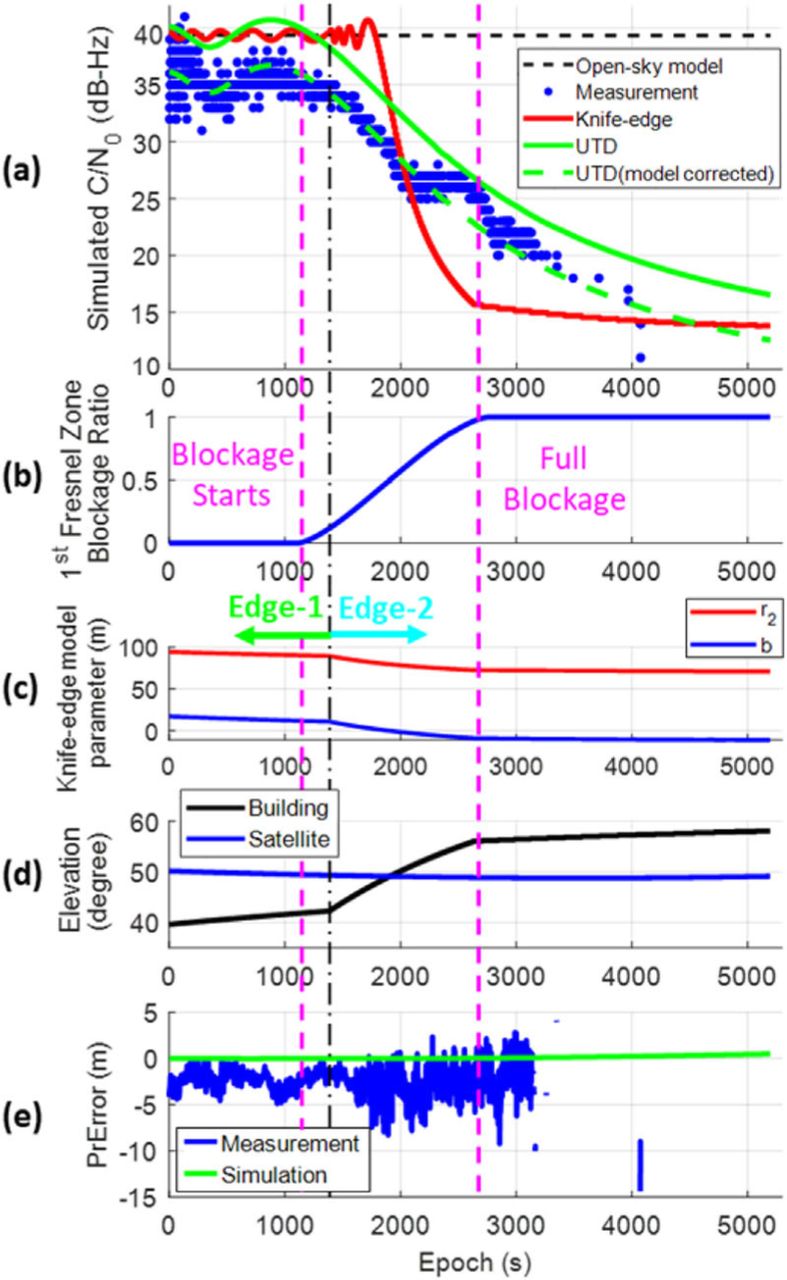
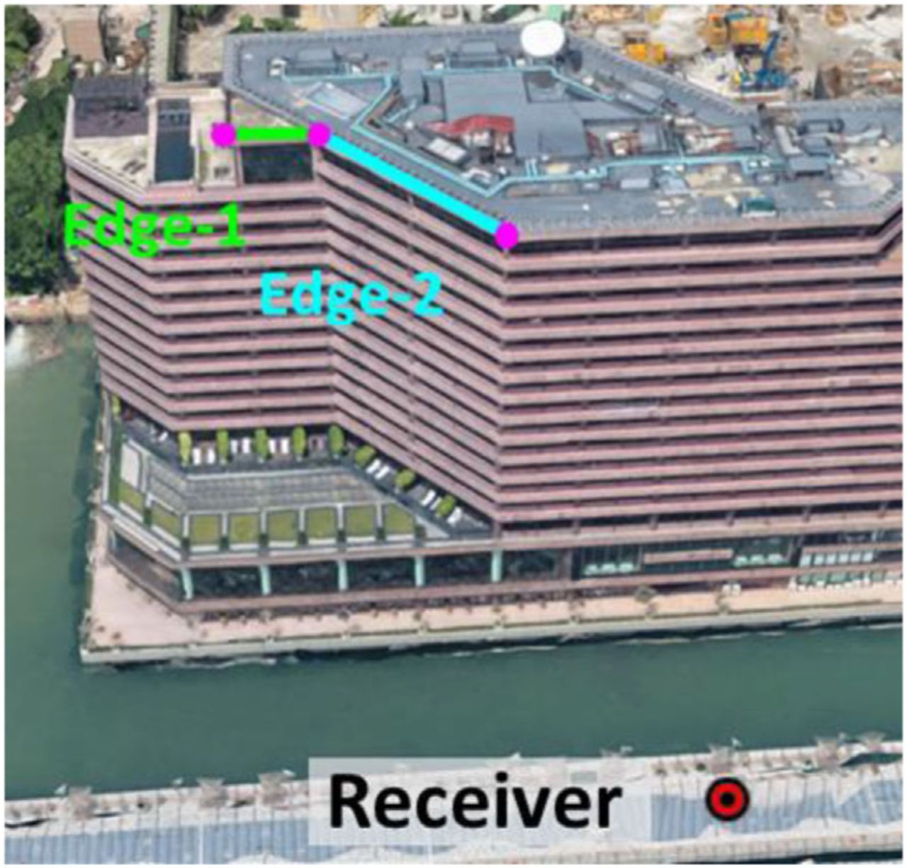
For satellite B10 in the one-side building scenario, diffracted by an oblique building edge (not perpendicular to the LOS vector), the simulation results are shown in Figure 10. In this scenario, the elevation angle of the building edge on the satellite’s azimuth angle is rapidly increased during the satellite movement. Consequently, the conventional knife-edge model also shows a rapid drop in the 𝐶∕𝑁0 simulation, which is inconsistent with the real measurements. Noted that the fluctuation of the simulated 𝐶∕𝑁0 from the knife-edge model is significantly changed at the epoch 1385. This is because the geometric parameters 𝑟2 and 𝑏 for the knife-edge model are under the transition from Edge-1-related to Edge-2-related (as shown in Figure 11), further influencing the switching frequency of the constructive/destruction interferences. On the other hand, by considering the three-dimensional (3D) angle in diffraction, the signal attenuation by UTD is slower, which is more similar to the real measurements. Notice that the simulated 𝐶∕𝑁0 by UTD has a bias compared with the measurement. It is because the open-sky model may have a constant error when predicting the 𝐶∕𝑁0 of the unobstructed signal. Analogous to the adjustment for unexpected interferences in (Nicolás et al., 2012), after manually adjusting the UTD simulation with -4 dB-Hz, the UTD (model corrected) simulation result is consistent with the real measurement. Moreover, the UTD can simulate the 𝐶∕𝑁0 fluctuation of the real measurement before attenuation, which is described as the interference between the LOS and the diffracted field. After the first Fresnel zone is entirely blocked, the diffracted signal remains available for a certain period. Therefore, the reception of those severely attenuated signals from diffraction may be more often than expected, which relates to the configuration of the receiver and antenna. The criteria of an unavailable signal based on the complete blockage of the first Fresnel zone is valid for geodetic setups, but not appropriate for low-cost setups. Similar to the result of satellite G27, the pseudorange error from simulated diffraction is only a few decimeters. Meanwhile, the DD-estimated pseudorange error from the measurement is dominated by the noises from the master satellite or receiver tracking loop and has no obvious error from diffraction delay. The pseudorange error analysis from G27 and B10 verify the assumption that the pseudorange error due to the diffraction delay is negligible compared to the 𝜎𝑈𝐸𝑅𝐸 for most practical cases. The diffraction influence on the pseudorange error is mainly the increment of tracking loop noise due to the signal attenuation.

The diffraction simulation results for satellite B10 in one-side building scenario, including: (a) comparison of the 𝐶∕𝑁0 between simulations and measurements, the UTD (model corrected) denotes the simulation with a -4 dB-Hz correction on the open-sky 𝐶∕𝑁0 model; (b) the blockage ratio of the first Fresnel zone; (c) the values of the geometric-related parameter 𝑟2 and 𝑏 during the knife-edge model simulation; (d) the elevation angles of satellite and building edge; and (e) the pseudorange error from simulated diffraction and real measurement

The demonstration of the involving building edges in the knife-edge model simulation during the transition on epoch 1385
5.3 Validation on surrounded by buildings scenario
For the satellite G13 in the surrounded by buildings scenario, its diffraction simulation results from the knife-edge model and the UTD that are compared with real measurements in Figure 12. Before the first Fresnel zone is entirely blocked, the simulated 𝐶∕𝑁0 has the same trend compared with the real measurement, but with a certain bias. This bias is, again, caused by the inaccurate open-sky model. However, after the first Fresnel zone is entirely blocked, the signal is not only still available, but also with a high 𝐶∕𝑁0 value. During this period, the corresponding pseudorange errors raise to over 50 meters, which is apparently larger than the typical pseudorange error within a dozen meters from diffraction delay or tracking loop noise. By using a popular ray-tracing technique for reflections (Hsu et al., 2016), a valid reflection path with nearly 50 meters delay is found in the later period of the experiment. Although the ray-tracing found no valid reflection around epoch 3,500-5,300, the measurement still has a typical reflection-related feature that the pseudorange contains an enormous positive delay. Therefore, as another frequently occurring effect in the urban area, the reflection interference needs to be considered and combined with the diffraction interference in order to achieve a good GNSS 𝐶∕𝑁0 and pseudorange simulation in dense urban scenarios.

The diffraction simulation results for satellite G13 in surrounded by buildings scenario, including: (a) comparison of the 𝐶∕𝑁0 between simulations and measurements; (b) the blockage ratio of the first Fresnel zone; and (c) the pseudorange error from measurement, diffraction simulation and the reflection effect simulated by the ray-tracing
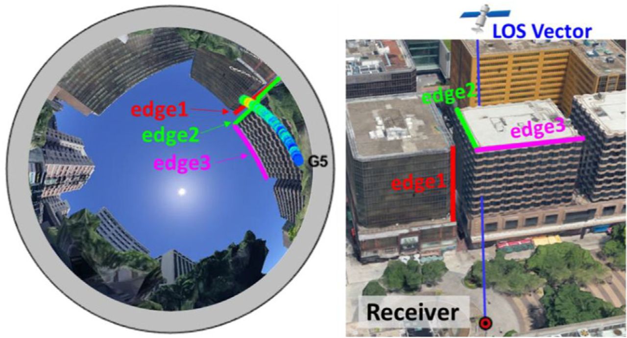
For the satellite G05 in the surrounded by buildings scenario, it experiences a transition involving three building edges, as shown in Figure 13. Therefore, the UTD simulation is based on the superposition of the diffracted fields from three involving building edges and the unobstructed field when the satellite is LOS. The diffraction simulation and real measurements are demonstrated in Figure 14, including the 𝐶∕𝑁0 simulation result of each individual diffracted field during UTD. Similar to the result of G13, the ray-tracing reflection simulation is also employed to find valid reflected signals during the experiment. The corresponding reflection delay is shown in Figure 14 (d). Although the simulation from the knife-edge model correctly reflects the rise of 𝐶∕𝑁0 when the satellite is LOS between the building gap, the change is too rapid since it only considers the building elevation angles. On the other hand, the UTD approach considers all three adjacent edges related to the diffraction in the manner of the superposition of multiple diffracted fields. The UTD simulation result is smoother than the knife-edge model and more consistent with the real measurement.

The skyplot of satellite G05 with a transition involving three different building edges in surrounded by buildings scenario
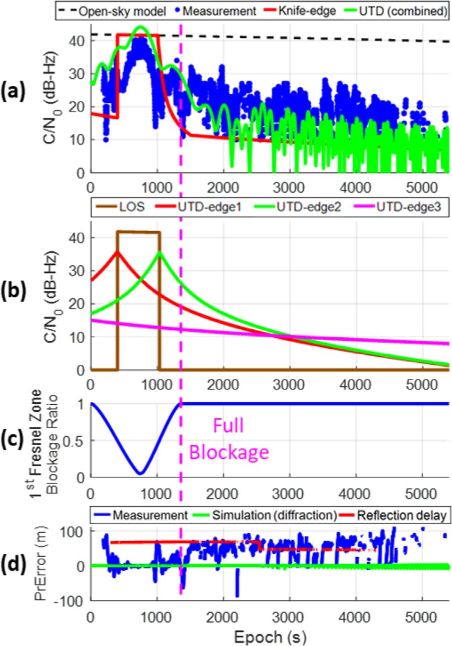
The diffraction simulation results for the satellite G05 in surrounded by buildings scenario, including: (a) comparison of the 𝐶∕𝑁0 between measurements and the simulations from knife-edge model and UTD combining multiple diffracted fields; (b) The individual simulation result of each involving diffraction field; (c) the blockage ratio of the first Fresnel zone; (d) the pseudorange error from measurement, diffraction simulation, and the reflection effect simulated by the ray-tracing
From the 𝐶∕𝑁0 of each diffracted field in Figure 14 (b), the overall field strength is dominated by the diffraction on edge1 when the satellite is blocked by the edge1-corresponded building. Then, the satellite is moving away from edge1 and becomes LOS for the receiver, which increases the 𝐶∕𝑁0 by considering the unobstructed field. As the satellite moving to the center of the building gap, the first Fresnel zone is almost without blockage, resulting in a high 𝐶∕𝑁0 close to an open-sky signal. Consistently, the 𝐶∕𝑁0 from the real measurement is also increased to the level of the open-sky model during this period. Besides diffractions, the measurement could also be degraded by the reflected signal, such as the enormous pseudorange error at around epoch 1,000, which is probably introduced by the reflected signal traced in Figure 15 (a). After that, the total field is dominated by the diffraction from edge2 when it approaches edge2. The total field decays after the blockage from edge2. Finally, the satellite is moving closer to edge3 rather than edge2, switching the dominance of the diffraction to edge3. As a result, the overall 𝐶∕𝑁0 simulation has a flatter decay in the final stage. However, the 𝐶∕𝑁0 plot of each diffracted field only demonstrates the amplitude of the signal, whereas each signal also has a different phase. The phase differences between different signals will introduce constructive or destructive interferences, leading to a fluctuation in the overall 𝐶∕𝑁0 simulation result in Figure 14 (a). As the results in the later period shows, such fluctuation becomes more significant when each signal has a similar amplitude. Noted that the 𝐶∕𝑁0 from the real measurement in the later stage is higher than the simulation. It is probably due to the reception of the signals reflected from other buildings, since an enormous pseudorange error is observed at the same period with a magnitude similar to the delay of the reflected signal found by ray-tracing in Figure 15 (b). In brief summary, the UTD can appropriately simulate the diffraction of the GNSS signal and the corresponding 𝐶∕𝑁0 attenuation and even be applicable during the transition involving multiple building edges.
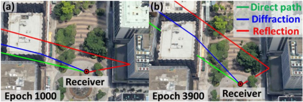
The ray-tracing simulation result of satellite G05 at epoch 1,000 and 3,900 during the experiment
5.4 Building model accuracy
Besides testing the consistency between the UTD simulation and real measurements, the influence of building model accuracy on the UTD is also worthy of analysis. Among all the geometrical parameters used in the UTD, the elevation angle of the building edge has the highest impact on the diffraction result since it controls the major parameter 𝜙 in Equations (7)-(10). The impact of the building model accuracy is evaluated based on the UTD simulation of satellite G08 in the one-side building scenario. The building introducing diffraction effect is around 34 meters away from the receiver with 60 meters height, corresponding to around the 60 degrees building elevation angle. Here, we manually assign ±2◦ error on 𝜙 in the building model when evaluating the influence of the building model accuracy for the UTD, which is equivalent to around a 5 meters building height error or around a 3 meters building distance error. As Figure 16 shows, the diffraction simulation results from UTD(±2◦) with ±2◦ error on the elevation angle of the building edge are compared with UTD(original), the original simulation without manually assigned error, and the real measurement. Compared with UTD(original), UTD(+2◦) occurs diffraction attenuation earlier, due to a larger elevation angle of the building edge and earlier blockage of the first Fresnel zone. On the contrary, UTD(−2◦) with a lower edge elevation angle will have a delayed attenuation from diffraction. Moreover, the building accuracy has a greater influence on the first Fresnel zone blockage ratio when the satellite is adjacent to the edge (the satellite elevation angle is close to the building elevation angle). In other words, the diffraction simulation is more sensitive to the error on the building edge when the satellite is closer to the edge. The building model error in height direction could also introduce error on the elevation angle of the edge, but related to the distance between building and receiver. For example, 1m height error only introduces 0.28◦ error on elevation angle for the 25m height building 200m away, but introduces 1.12◦ error on elevation angle when the building is 25m away. Therefore, the diffraction simulation is more sensitive to the dimensional model error from a nearby building. In general, the building model error will introduce an error on the simulation result as an overall shift on time series, due to the advance or delay of the first Fresnel zone blockage. This characteristic is also applicable to the knife-edge model approach.
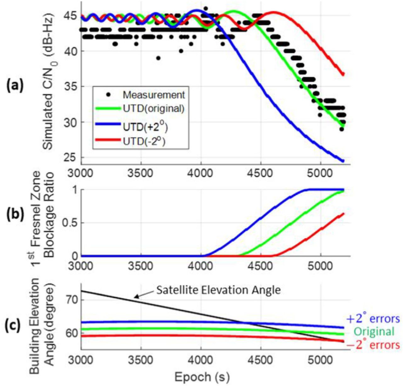
The influence of building model inaccuracy on the UTD simulation results for satellite G08 in one-side building scenario, including: (a) comparison of 𝐶∕𝑁0 between measurements and simulations, where UTD(±2◦) denote the simulation with ±2◦ errors on the elevation angle of the building edge and UTD(original) denotes the simulation without any assigned error on building edge; (b) the blockage ratio of the first Fresnel zone; and (c) the elevation angles of the satellite and the elevation angles of the building edges in the azimuth direction of the satellite
5.5 Comparison between the knife-edge and the UTD models
The computational load of these two methods during the simulations on different satellites is demonstrated in Figure 17. For the diffraction simulation of satellite G27, B10, G08, and G13 only involving a single building edge, both methods averagely cost around 0.001 seconds for one epoch simulation, while the UTD costs a slightly larger computation. By dividing the total computation load into the ray-tracing process and the attenuation model process, it is clear that most of the computations are spent on employing the ray-tracing to obtain geometrical parameters for each model. The UTD requires much more geometrical parameters than the knife-edge model, resulting in a higher computation for its ray-tracing process. Moreover, during the simulation of G05 in a complex environment, the UTD considers the combination of three different diffracted fields. Hence, the UTD needs to apply ray-tracing on three building edges, making the computation load three times higher than the knife-edge model. Besides the computational load, the UTD has better accuracy than the knife-edge model on the 𝐶∕𝑁0 simulation of the diffracted signal, since it considers the addition of geometrical details in 3D. The root-mean-square (RMS) error of the 𝐶∕𝑁0 simulation result compared to the real measurement for each satellite is shown in Table 1. Besides the similar results from G08 and G13, the UTD has less simulation error than the knife-edge model, noted that the simulation is based on the low-cost receiver with higher noise than the geodetic receiver, resulting in a small error even in the open-sky scenario. Both methods have over 8 dB-Hz 𝐶∕𝑁0 modeling RMS error in the urban scenario, possibly due to the reflection interferences after the first Fresnel zone has been fully blocked. For the UTD approach before the full blockage of the first Fresnel zone, the standard deviation of the 𝐶∕𝑁0 modeling errors for G13 and G05 in the urban area are 2.5 meters and 3.4 meters, which still show good consistency with the real measurements. Finally, the UTD simplifies the diffraction as a local effect. This idea can be employed to describe the pseudorange error caused by diffraction as a delay introduced by a specific signal traveling through the diffraction point. On the other hand, the knife-edge model based on the integral is too complicated to simulate the pseudorange error. The characteristics of the knife-edge model and the UTD on urban GNSS diffraction simulation are summarized in Table 2.

The computational load of diffraction simulation based on the knife-edge model and the UTD for different scenarios. The total computation load of each method is divided into two parts: the ray-tracing estimation process (unshaded area) and the attenuation modeling process (shaded area)
The root-mean-square error (unit: dB-Hz) of the C/N0 simulation of the diffracted signal
Characteristics of diffraction simulation methods
5.6 Diffraction effect verification by the correlator output
Besides evaluating the diffraction modeling performance with the collected measurements, it is also necessary to verify whether those diffracted measurements are legitimate. For example, even when a satellite becomes unavailable to the receiver, the corresponding measurements may still be generated from the tracking loops until the lock detector concludes its disappearance. Such illegitimate measurements due to the delay of the disappearance conclusion could result in a degradation similar to that of a diffraction effect. A feasible way to verify the legitimacy of the available measurements during diffraction is to identify the navigation bit stream from the correlator outputs corresponding to those measurements. Therefore, an additional experiment is conducted in the one-side building scenario to simultaneously collect the receiver independent exchange format (RINEX) data and the correlator outputs data during the diffraction effect. Since the ublox EVK-M8T receiver does not support the correlator outputs, we employ another low-cost GNSS receiver, a smartphone, to collect the correlator outputs simultaneously at the same location.
The experimental results are shown in Figure 18, including the simulation results, the available measurements from the ublox EVK-M8T, and the prompt in-phase and quadrature phase plot from the smartphone corresponding to four labeled 1-minute periods. Consistent with the preceding analysis, the UTD achieves adequate simulation performance on the diffraction effect. During periods 1 and 2, the first Fresnel zone of the satellite signal is not fully blocked. The corresponding I-Q plot shows a clear ring, which verifies the existence of the navigation message. Note that the smartphone here employs the frequency locked loop (FLL) in the tracking loop, which makes the navigation message form a ring due to the energy spreading on Q. For the noise without the navigation message, the corresponding I-Q plot will be concentrated in the center. During period 3, with a fully blocked first Fresnel zone, the available 𝐶∕𝑁0 measurements are under the degradation consistent with the UTD simulation. Meanwhile, the existence of the navigation message can be observed by the ring-like I-Q plot from the correlator outputs data at the same location, which verifies the legitimacy of those available measurements. Even during the later period 4, the corresponding I-Q plot is a bit sparse in the center, which could indicate that the navigation message may still be there. In summary, verified by the correlator outputs indirectly, the UTD can adequately model the diffraction degradation in the legitimate measurements from a low-cost receiver.

The diffraction simulation result for satellite G16 in the one-side building scenario, including: (a) comparison of the 𝐶∕𝑁0 from the UTD simulation and real measurements; (b) the blockage ratio of the first Fresnel zone; (c) the elevation angles of the satellite and the elevation angles of the building edge in the azimuth direction of the satellite; (d) the pseudorange error from simulated diffraction and real measurement; (e) the prompt I-Q plots of the correlator output from another low-cost receiver corresponding to four labeled 1-min periods
6 CONCLUSIONS AND FUTURE WORKS
The GNSS signal diffraction simulation based on the knife-edge model and the UTD is interpreted in this study, including the aspects that required special consideration for GNSS, such as the geometrical simplification and polarization. Then, the procedures to simulate the diffracted GNSS measurements on 𝐶∕𝑁0 and pseudorange are presented in detail. The 𝐶∕𝑁0 of the diffracted signal is simulated based on the open-sky 𝐶∕𝑁0 model and the diffraction coefficient estimated by the geometrical parameters with the knife-edge model or the UTD. The diffracted pseudorange is simulated based on the multipath envelope model and the 𝐶∕𝑁0 ratio between the diffracted and the direct signal.
The performance of diffraction simulation is assessed through real experimental data in different urban scenarios. The simulated 𝐶∕𝑁0 of the diffracted GNSS signal from UTD is consistent with the real measurement, even when the signal undergoes a transition involving multiple diffraction sources. Due to the higher sensitivity of the low-cost receiver, its reception of the diffracted signals may be more often, even if the corresponding first Fresnel zone has been fully blocked. From both simulation and real measurement, the pseudorange error due to diffraction is negligible compared to the common noise. Moreover, the reception of reflected signals may occur in a scenario with multiple buildings. Besides the diffraction, the reflection of signals is also required to be considered for a better GNSS measurement simulation in the dense urban area. Compared to the knife-edge model, the UTD is more accurate, but requires a higher computational load, especially when considering multiple diffracted fields.
The GNSS diffraction simulation can fulfill the need for a realistic urban GNSS measurement simulator considering diffraction for various studies on the GNSS positioning in the urban area. Besides contributing to the GNSS simulator development, accurate diffraction modeling may also have the potential to improve the GNSS positioning performance, especially for the 3DMA GNSS. Most of the 3DMA GNSS techniques determine the user positioning through a simulation-measurement matching process. For example, the shadow-matching algorithm aims to find the candidate position with the simulated satellite visibility best matching the visibility estimation from real measurements. Similarly, the 3DMA GNSS ray-tracing aims to find the candidate position having the direct/reflected pseudorange simulations that best match the real measurements. The UTD model can extend the ray-tracing positioning by enriching the matching process with the diffraction measurement, which is another type of measurement that frequently occur in the urban area besides LOS and NLOS. Therefore, with more information to conduct the simulation-measurement matching process, diffraction modeling has the potential to improve the 3DMA GNSS positioning performance. However, the justification of this contribution needs rigorous methodology development as well as a comprehensive investigation, which will be regarded as the future works of this study.
Despite of the benefits, the current diffraction modeling method may still have the limitation to contribute the high precision application using the carrier phase measurements. The modeling of the phase shift is sensitive to the building model accuracy with a resolution in centimeter level, which is hard to be guaranteed by the current LOD-1 models. Moreover, for some cases, both the knife-edge and the UTD models could experience a certain simulation bias due to the limitation of the elevation-angle-based 𝐶∕𝑁0 regression model. This regression model may not always precisely represent the behavior of the obstructed signal strength, which relates to not only the satellite elevation angle but other factors as well.
HOW TO CITE THIS ARTICLE
Zhang G, Hsu L-T. Performance assessment of GNSS diffraction models in urban areas. NAVIGATION. 2021; 68(2):369–389. https://doi.org/10.1002/navi.417
ACKNOWLEDGMENTS
This work was supported by PolyU RISUD EFA fund on the project BBWK, “Resilient Urban PNT Infrastructure to Support Safety of UAV Remote Sensing in Urban Regions.” The authors would like to acknowledge of Dr. Bing Xu on his contribution to instruct the first author on the use and knowledge of GNSS SDR.
APPENDIX A: NOMENCLATURE
APPENDIX B: EXAMPLE OF THE DLL TRACKING LOOP NOISE
The pseudorange noise from the GNSS receiver code tracking loop, delay lock loop (DLL), is normally dominated by the thermal noise code tracking jitter related to the 𝐶∕𝑁0 of the GNSS measurement. The measurement with a lower 𝐶∕𝑁0 will have a higher DLL noise, resulting in a noisier pseudorange measurement. For the C/A code with BPSK modulation, the relationship between the thermal noise code tracking jitter and the 𝐶∕𝑁0 can be derived as follows (Kaplan & Hegarty, 2017):
 B1
B1
where 𝜎𝑡𝐷𝐿𝐿 is 1-sigma thermal noise code tracking jitter, 𝑑 is the early-to-late correlator spacing (unit of chip), 𝐵𝑓𝑒 is the front-end bandwidth, 𝑅𝑐 is the chip rate, 𝐵𝑐𝑜𝑑𝑒 is the code loop noise bandwidth, 𝑇𝑖 is the predetection integration time, and 𝑇𝑐 is the chip period. A numerical example of the relationship between 𝜎𝑡𝐷𝐿𝐿 and the 𝐶∕𝑁0 is shown as Figure B1. The GNSS measurement with 25 dB-Hz 𝐶∕𝑁0 may have roughly 5 meters pseudorange noise (1-sigma) during the DLL tracking loop.
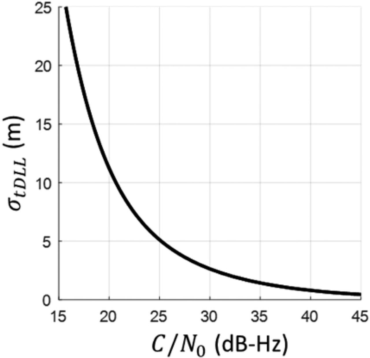
An example of the relationship between the thermal noise code tracking jitter and the 𝐶∕𝑁0. The values of the corresponding parameters are 𝑑 = 1 chip, 𝐵𝑓𝑒 = 2.046 MHz, 𝑅𝑐 = 1.023 MHz, 𝐵𝑐𝑜𝑑𝑒 = 0.2 Hz, 𝑇𝑖 = 0.02 s
Footnotes
Funding information
Research Institute for Sustainable Urban Development, Hong Kong Polytechnic University, Grant/Award Number: Resilient Urban PNT Infrastructure to Support Safety of UAV Remote Sensing in Urban Regions
- Received July 12, 2020.
- Revision received February 15, 2021.
- © 2021 The Authors. NAVIGATION published by Wiley Periodicals LLC on behalf of Institute of Navigation.
This is an open access article under the terms of the Creative Commons Attribution License, which permits use, distribution and reproduction in any medium, provided the original work is properly cited.


Jump to section
- Article
- Abstract
- 1 INTRODUCTION
- 2 KNIFE-EDGE DIFFRACTION MODEL
- 3 UNIFORM GEOMETRICAL THEORY OF DIFFRACTION
- 4 GNSS DIFFRACTION SIMULATIONS
- 5 EXPERIMENTAL VALIDATIONS
- 6 CONCLUSIONS AND FUTURE WORKS
- HOW TO CITE THIS ARTICLE
- ACKNOWLEDGMENTS
- APPENDIX A: NOMENCLATURE
- APPENDIX B: EXAMPLE OF THE DLL TRACKING LOOP NOISE
- Footnotes
- REFERENCES
- Figures & Data
- Supplemental
- References
- Info & Metrics
Related Articles
Cited By...
- No citing articles found.