

Abstract
A new global navigation concept is studied that relies on carrier Doppler shift measurements from a large LEO constellation. This system could provide an alternative to pseudorange-based GNSS. The concept uses a high-fidelity model of received carrier Doppler shift. This model is used in a point-solution batch filter that simultaneously estimates eight unknowns: the three position vector components, receiver clock offset, three velocity vector components, and receiver clock offset rate. The filter uses eight or more measured Doppler shifts in its least-squares fit. A generalized Geometric Dilution of Precision (GDOP) analysis indicates that absolute position accuracies on the order of 1-5 meters and absolute velocity accuracies on the order of 0.01 m/sec to 0.05 m/sec may be achievable if the range-rate precision of the Doppler shift measurements is 0.01 m/sec. These accuracies are comparable to current pseudorange-based GNSS. Clock offset accuracy is on the order of 0.0001 to 0.0010 sec 1-𝜎.
1 INTRODUCTION
This effort seeks an alternative, or backup, to standard Global Navigation Satellite Systems (GNSS) that operate in Medium Earth Orbit (MEO) and above– systems such as GPS, GLONASS, Galileo, and BeiDou. These systems have vulnerabilities to spoofing and jamming partly because their signals are weak and partly because they use low numbers of expensive satellites with long lifespans, which makes upgrading them slow and expensive.
The present study seeks to develop a system that achieves a full 4-Dimensional (4D) Position/Navigation/Time (PNT) capability by using passive reception of downlink signals from large LEO constellations. It seeks to exploit the various plans that exist to field large constellations of Low Earth Orbit (LEO) satellites such as OneWeb, Starlink, and Kuiper.
OneWeb has built and launched a number of satellites already and had plans at one time to field a LEO constellation with 720 satellites in 18 nearly-polar orbital planes (FCC Report, 2017). Although the company went bankrupt, it has since been bought, and there are now renewed plans to field the constellation, perhaps with a GNSS capability added to the original satellite design. SpaceX has been launching satellites for its Starlink constellation. One plan calls for an initial constellation of 1,600 LEO satellites that eventually expands to 2,825 satellites (FCC Report, 2016). Amazon has plans for an 1,156 satellite LEO constellation called Kuiper (FCC Report, 2019).
It is not anticipated that such constellations will support pseudorange-based navigation for two reasons: First, they will not carry atomic clocks. Second, they will not broadcast downlink signals that support pseudorange measurements through a calibrated connection between transmission time tags and transmitter clock time.
Therefore, the present study seeks to perform navigation using carrier Doppler shift as the only navigation observable. Carrier Doppler shift is generally easy to measure from a radio signal that carries digital data. This author has experience measuring carrier Doppler shift from signals that use BPSK, QPSK, and OFDM modulation schemes, [e.g., see Psiaki & Slosman (2019)]. They have proven amenable to precise measurement of carrier Doppler shift.
Similar to pseudorange-based GNSS, a point-solution methodology is developed for Doppler-shift-based GNSS. Instead of using four or more pseudorange measurements to determine 3-Dimensional (3D) position and receiver clock offset, the new method uses eight or more carrier Doppler shift measurements to determine 3D position, receiver clock offset, velocity, and receiver clock offset rate. The need for measurements from eight or more satellites arises because all eight of these unknowns appear in any navigation-grade model of carrier Doppler shift.
The term TRANSIT on steroids in this paper’s title refers to the TRANSIT Navigation System that was developed in the 1950s and 1960s (Parkinson, 1996). The TRANSIT system consisted of less than a dozen LEO satellites. Typically a user could receive a signal from one satellite at a time, perhaps with gaps of an hour or more when no satellites were visible. The user receiver measured carrier Doppler shift from the broadcast TRANSIT signal, as is done in the present work. If the user velocity and altitude were known, as for a TRIDENT submarine at periscope depth operating with a very stable Inertial Navigation System (INS), then a position fix could be obtained from a single satellite pass. The accuracy was on the order of 200 meters.
With the advent of large LEO constellations and the simultaneous visibility of more than eight satellites, it may be possible to use the principles of TRANSIT to much better effect: There would be no availability gaps, no need to know velocity or altitude a priori, and no need for an INS. TRANSIT on steroids might be able to navigate smartphones and drones, not just ballistic missile submarines.
Other researchers have considered the possibility of using large LEO constellations for navigation, [e.g., (Benzerrouk & Fang et al., 2019; Benzerrouk & Nguyen et al., 2019; Gutt etal., 2018; Iannucci & Humphreys, 2020; Kassas et al., 2019; Khalife & Kassas, 2019a; Khalife & Kassas, 2019b; Morales et al., 2019; Morales-Ferre et al., 2020; Racelis et al., 2019; and Reid et al., 2018)]. Some studies have considered carrier Doppler shift or beat carrier phase, which is the negative time integral of Doppler shift. A subset of the relevant research has examined the use of Doppler shift in conjunction with pseudorange, as in Kassas et al. (2019). INS aiding has been considered in some papers, such as in (Benzerrouk & Fang et al., 2019) and (Morales et al., 2019).
The only paper known to this author that considered a full navigation capability using only carrier Doppler shift measurements in a point solution is Morales-Ferre et al. (2020). That paper’s system, however, does not provide a full navigation capability because it assumes that the user receiver’s velocity and clock offset are both zero. Thus, the present paper is the first to consider Doppler-only navigation without any assumptions about velocity or receiver clock offset and without the need for aiding from an Inertial Navigation System (INS) or for pseudorange data. It is the first to show that receiver clock offset is observable simultaneously with 3D position, 3D velocity, and receiver clock offset rate solely from carrier Doppler shift measurements.
This paper makes three contributions to the subject of carrier-Doppler-shift-based navigation using signals from large LEO constellations: First, it develops three useful carrier Doppler shift measurement models. Second, it develops a point-solution algorithm for determining position, receiver clock offset, velocity, and receiver clock offset rate from eight or more carrier Doppler shift measurements. This algorithm solves a nonlinear least-squares estimation problem. This paper examines the performance of the new point-solution algorithm on simulated data, including data that contain un-compensated satellite ephemeris errors and transmitter clock frequency offsets. Third, this paper develops a generalized Geometric Dilution of Precision (GDOP) analysis for this concept, presenting GDOP maps for several constellations, and examining constellation characteristics that are important to achieving good performance with such a system.
The analyses and results of this paper are presented in seven main sections followed by a summary and conclusion. The second section presents three models of carrier Doppler shift. The third section reviews four large LEO constellations in order to assess their potential suitability for carrier-Doppler-shift-based navigation. The fourth section develops a batch least-squares filter for determining point solutions of position, clock offset, velocity, and clock offset rate based on eight or more measured carrier Doppler shifts. The fifth section applies this batch filter to simulated truth-model data in order to study the navigation performance of the system. The sixth section develops a generalized GDOP analysis for Doppler-based navigation. The seventh section uses this new GDOP metric to explore the potential performance of several large LEO constellations. The eighth section discusses other considerations that are important to such a system which have not been addressed in the present study. The ninth section gives a summary of this paper’s results and presents its conclusions.
2 CARRIER DOPPLER SHIFT MEASUREMENT MODELS
2.1 Doppler shift from the time derivative of accumulated delta range
The measured carrier Doppler shift equals the negative time derivative of the accumulated delta range divided by the carrier wavelength:
 1
1
where 𝐷𝑗 is the measured carrier Doppler shift from the 𝑗th GNSS satellite in Hz, 𝜆 is the nominal wavelength in meters,  is the accumulated delta range in meters, and 𝑡𝑅 is the erroneous receiver clock time. It is related to the true signal reception time 𝑇𝑅 and the receiver clock offset 𝛿𝑅 as follows:
 2
2
The accumulated delta range can be modeled as follows:
 3
3
where  is the unknown user receiver position vector in Earth-Centered/Earth-Fixed (ECEF) Cartesian coordinates–typically WGS-84 coordinates,
  is the known orbital position time history of the 𝑗th GNSS satellite in ECEF coordinates, 𝜔𝐸 is the Earth’s rotation rate,
  is the propagation time of the signal from the satellite to the receiver, 𝛿𝑗 is the satellite clock offset,
  is the signal delay due to the neutral atmosphere (mostly due to the troposphere),
  is the time-equivalent carrier phase advance that is caused by dispersive refraction in the ionosphere, and 𝛽 is the bias on the measured beat carrier phase.
Although not explicitly noted in Equation (3), the signal propagation delay implicitly depends on  , 𝛿𝑅, and 𝑡𝑅 because it must be computed by solving the following delay equation:
 4
4
Note that the ionosphere term acts as a delay in this equation.
The troposphere delay term  and the ionosphere advance/delay term
  also depend on
  , 𝛿𝑅, and 𝑡𝑅. This dependence comes partly through the Line-of-Sight (LOS) unit direction vector from the satellite to the receiver:
 5
5
This unit vector affects the elevation angle through the troposphere and the ionosphere pierce-point location and zenith angle. The receiver location  also affects the ionosphere pierce-point location directly.
The 3×3 direction cosines matrix:
 6
6
appears in Equations (3) through (5). It compensates for the rotation of the ECEF coordinate frame while the signal travels from the satellite to the receiver.
2.2 Analytic carrier Doppler shift model
Equations (1) through (6) can be used to derive an analytic carrier Doppler shift model. If one ignores the time derivatives of the troposphere and ionosphere terms, then this model takes the form:
 7
7
after multiplication of Equation (1) on both sides by −𝜆, which transforms to the range-rate equivalent of the carrier Doppler shift. A derivation of this equation is given in the appendix.
The new quantities introduced in this model are the unknown receiver velocity  , the unknown receiver clock offset rate 𝑑𝛿𝑅/𝑑𝑇𝑅, the known ECEF satellite velocity at the time of transmission (but transformed to the ECEF frame of the time of reception)
  , which is the time of signal transmission, the satellite clock offset rate
  , and
, and  , which is a term that arises due to the time rate of change of the propagation delay
  .
.
The formula for the satellite velocity is:
 8
8
The  term takes the form:
 9
9
where  is the Earth’s rotation rate vector given in ECEF coordinates.
The carrier Doppler shift model in Equation (7) has some terms in common with the model given in (Aumayer & Petovello, 2015). The present model, however, is more complete and explicit in its characterizations of the effects of clock offset rates, satellite velocity, and the time rate of change of  .
.
The Doppler shift model in Equation (7) has been used extensively by the author to solve for velocity  and range-rate-equivalent receiver clock offset rate 𝑐(𝑑𝛿𝑅/𝑑𝑇𝑅) by using the carrier Doppler shift measurements from four or more GPS satellites. This velocity solution assumes that the receiver position
  and the receiver clock offset 𝛿𝑅 have already been determined from a pseudorange solution. The values of
  and 𝛿𝑅 are needed in order to compute the terms
  , and 𝑑𝛿𝑗/𝑑𝑇𝑗 that appear in Equation (7). Peraxis accuracies on the order of 0.01 m/sec RMS have been demonstrated. Velocity biases are negligible.
The accuracy is good enough to enable mapping of a vehicle’s relative route via simple quadrature integration of the velocity solution time history that results from using this model. Relative position accuracies on the order of 1 meter or better have been observed after 5 to 10 minutes of velocity integration. These levels of accuracy were obtained by the author in preparation of a university course and by students who completed the data-processing lab portion of that course using recorded carrier Doppler shift and pseudorange data from a survey-grade Magellan receiver mounted on an automobile. The foregoing statements represent the first public release of these accuracy results.
The dependence of the terms  , and
, and  on position and receiver clock offset is a liability when using carrier Doppler shift measurements for velocity estimation. A pseudorange-based navigation solution is needed to overcome this liability.
In the present context, however, this dependence is an asset. It makes position and receiver clock offset simultaneously observable with velocity and clock offset rate. The minimum number of needed signals grows from four to eight in this situation because of the increased number of unknowns that must be estimated. As will be shown in the section on generalized GDOP analysis, this method’s accuracy depends on the rapidity with which the GNSS satellites pass over the receiver. That is why this technique will not work well with MEO GNSS satellites even when carrier Doppler shift data are available from eight or more of them.
2.3 Carrier Doppler shift model based on finite differencing of accumulated delta range
Although the Doppler shift model in Equation (7) works well for velocity and clock offset rate estimation when position and clock offset are known, it is not clear that it will work well for the present application. It’s performance may be lacking due to its neglect of the time derivatives of the troposphere and ionosphere terms.
Therefore, an alternate carrier Doppler shift model has been developed for use in the joint estimation of position, receiver clock offset, velocity shift, and receiver clock offset rate. One could develop an analytic model that included the effects of the non-zero time derivatives of the troposphere and ionosphere terms. The complexity of such a derivation, however, would be considerable. Instead, a suitable model has been developed based on a 5-point finite difference calculation that numerically computes the time derivative of the accumulated delta range.
This model starts with the assumption that there already exists a function which computes the model of the accumulated delta range given in Equation (3). The accumulated delta range model’s calculations are assumed to include solution of propagation delay Equation (4) for  and model-based calculation of the troposphere and ionosphere terms
  and
and  . Thus, it captures all of the ways in which
  depends on
  , 𝛿𝑅, and 𝑡𝑅.
The 5-point finite difference formula for the accumulated delta range rate uses the accumulated delta range model to perform the following calculation:
 10
10
where Δ𝑡𝑅 is the nominal finite difference interval of the erroneous receiver clock time 𝑡𝑅 and:
 11
11
is shorthand for the unknown receiver clock offset rate. The true reception time’s corresponding finite difference interval is  , which accounts for the presence of the factor
  in several parts of this formula. Note that this 5-point finite-difference formula only contains four weighted terms because it uses a weighting of zero for the middle term, (i.e., the term with zero time offset).
The accumulated delta range rate model in Equation (10) is substituted into Equation (1) to yield the carrier Doppler shift model that forms the basis of point solutions for position, clock offset, velocity, and clock offset rate. This finite-difference model has been employed successfully by the author in a navigation system that uses carrier Doppler shift data from the Iridium constellation in addition to data from other sensors. A finite difference interval in the range 0.1 sec ≤ Δ𝑡𝑅 ≤ 0.25 sec works well.
2.4 Simplified analytic carrier Doppler shift model for use in GDOP analysis
The preceding Doppler shift models are too complicated for use in a Geometric Dilution of Precision (GDOP) analysis. A GDOP analysis only needs to consider the dominant ways in which the unknowns affect the measurements. Its model must characterize how errors in the measurements are related to errors in the estimates of the unknown quantities. Second-order effects, while important in the calculation of an actual navigation solution, typically have a negligible impact on a GDOP calculation.
Several small effects have been neglected in order to simplify the carrier Doppler shift model for use in the GDOP analysis. First, the effects of the troposphere and the ionosphere have been omitted. They do not have a large impact on the sensitivity of the measurements to small perturbations of the unknowns. Omission of the atmospheric terms allows Equation (7) to be the starting point for developing a simplified model.
Three additional simplifications substitute the value 1 in place of three terms in Equation (7) that nearly equal 1. The three substitutions are:
 12
12
The first two of these approximations are typically accurate to seven or more significant digits due to the stability of the transmitter and receiver clocks. The last of these approximations is accurate to more than four significant digits due to the low speed of the satellite relative to the speed of light.
Given the foregoing approximations, the simplified carrier Doppler shift model takes the form:
 13
13
This is the model that will be used to develop a generalized GDOP analysis. It is suitable only for that purpose. It should not be employed to compute point solutions using this paper’s new navigation method. It should not even be used for determining velocity and receiver clock offset rate when position and clock offset are known from a pseudorange-based navigation solution.
3 REVIEW OF LARGE LEO CONSTELLATIONS AND THEIR SUITABILITY FOR DOPPLER-ONLY PNT
Several large LEO constellations exist, are being fielded, or are planned. These include the Iridium constellation, which is currently operational, OneWeb and Starlink, which each have satellites in orbit, and Kuiper, which has not yet progressed to the point of launching satellites.
Table 1 lists parameters of these constellations that are relevant to their suitability for Doppler-based navigation. The numbers for Iridium are common knowledge because the constellation has been operational for decades. The numbers for the other three constellations have been gleaned from (FCC Reports, 2016, 2017, 2019).
Characteristics of large LEO constellations
Newer information than that given in the cited documents is available from recent FCC filings for the OneWeb, Starlink, and Kuiper constellations. Some of the newer numbers differ from those in the table. A decision has been made to use the particular numbers cited below because there is no certainty that even the latest plans will be the final ones which get implemented. Rather than constantly chase the latest numbers, it seems reasonable for this initial study to lock in some representative constellation configurations and analyze them.
The final column of Table 1 provides an important metric of constellation suitability for Doppler-based navigation: the minimum number of visible satellites. Except for the Iridium constellation, each of these numbers has been deduced from four constellation visibility simulation snapshots on a 1o latitude by 1o longitude grid over the entire surface of the Earth–-except that the Starlink (initial) and Kuiper grids are restricted in latitude, as noted in the table’s footnotes.
Each simulation randomizes the constellation’s first orbital plane’s right ascension and that plane’s initial satellite’s argument of longitude. All other orbital plane right ascensions and satellite arguments of longitude are linked to these two datums. Therefore, the numbers in the last column represent good approximations of minimum guaranteed values 100% of the time for a clear sky view. A given constellation’s number needs to be eight or larger in order for the proposed system to be viable.
Therefore, the Iridium constellation alone cannot support the present concept. Typically a user receiver sees only a single satellite. It sees two satellites for a short period about once every 10 minutes. On rare occasions, a user receiver may see three or four satellites, but it will never see eight simultaneously except around the North and South poles.
The OneWeb, Starlink, and Kuiper constellations all appear to be viable because their minimum numbers of visible satellites are above eight. Note, however, that the initial Starlink deployment plan and the Kuiper plan do not include any high-inclination orbits. Therefore, these two configurations cannot guarantee the simultaneous visibility of eight or more satellites at locations within 25o or 30o of the North and South poles.
It might be best to use a combination of constellations if it is practical to design receivers for each constellations’ different signals. Perhaps a good design would use a combination of OneWeb to cover the polar regions and Kuiper to enhance performance in the mid-latitude and equatorial regions.
The numbers in the last column of Table 1 do not provide the final word on constellation suitability for Doppler-only navigation. Having a minimum of eight visible satellites is a necessary condition for the viability of this concept, but it is not a sufficient condition. A generalized GDOP analysis must be used in order to assess the likely performance of a particular constellation or combination of constellations.
4 POINT SOLUTIONS USING A BATCH LEAST-SQUARES FILTER
A point-solution algorithm has been developed to calculate a navigation fix from eight or more measured carrier Doppler shifts. This algorithm is the carrier-Doppler-shift analog of the algorithm that solves four or more pseudorange equations for the receiver position and clock offset in standard GNSS signal processing. The algorithm computes estimates of the position  , the receiver clock offset 𝛿𝑅, the velocity
  , and the receiver clock offset rate
  by solving the following nonlinear least-squares problem:
 14
14
The accumulated delta range time derivative model used in the numerator on the the right-hand side of the least-squares cost function is the finite-difference-based approximation given in Equation (10). The quantity  is the carrier Doppler shift measurement error standard deviation for the signal from the 𝑗th satellite given in Hz units. This cost function is a weighted sum of the squared errors in the carrier Doppler shift measurement model of Equation (1) after both sides of the model have been multiplied by 𝜆 to give the model in range-rate-equivalent form. The denominator term
  is the range-rate-equivalent measurement error standard deviation in units of m/sec for the 𝑗th satellite. It normalizes the corresponding residual error in the cost function. This normalized cost function is a negative log-likelihood function. Therefore, minimization of
  amounts to maximum-likelihood estimation.
The cost function in Equation (14) can be re-cast into the following standard weighted nonlinear least-squares form:
 15
15
where:
 16
16
is the 8×1 vector of unknown quantities that are to be estimated:
 17
17
is the 𝑁×1 measurement vector:
 18
18
is the 𝑁×1 nonlinear measurement model function, and:
 19
19
is the 𝑁×𝑁 measurement error covariance matrix.
This standard nonlinear least-squares problem is solved using the Gauss-Newton method (Gill et al., 1981). The Gauss-Newton method starts with a guess 𝒙𝑔. It linearizes the measurement model function 𝒉(𝒙) around each guess and solves the corresponding linearized least-squares problem using matrix methods in order to compute an increment to the current guess, Δ𝒙.
It next performs a line search along this direction to find a step length 𝛼 such that 𝐽(𝒙𝑔 +𝛼Δ𝒙) < 𝐽(𝒙𝑔). The line search uses simple bisection. It starts by trying 𝛼 = 1. It then scales 𝛼 down by successive factors of 1/2, as needed, until it finds a value that reduces the cost function. Finally, the old guess 𝒙𝑔 is replaced by the new guess 𝒙𝑔 +𝛼Δ𝒙, and the algorithm iterates until it converges. The line search for 𝛼 ensures robust convergence to a minimum.
A Gauss-Newton algorithm can have very slow convergence if its first guess starts too far away from the optimal solution. Another issue that can cause slow convergence is the possibility that the residual differences between 𝒚 and 𝒉(𝒙) at the optimal solution will be large enough to cause the linearized approximation of 𝒉(𝒙) to yield a poor prediction of how the cost function will change due to the solution increment Δ𝒙. Therefore, an important question about this batch least-squares algorithm concerns the speed with which it converges when starting far from the solution and in the vicinity of the solution.
The batch least-squares negative log-likelihood cost function can be used to compute an approximation of the estimation error covariance for this system. Suppose that:
 20
20
where 𝒙𝑜𝑝𝑡 is the optimal estimate that minimizes 𝐽(𝒙). This 𝑁×8 measurement model Jacobian matrix can be used to compute the following approximation of the Cramer-Rao lower bound for the estimation error covariance matrix:
 21
21
This matrix characterizes the precision of the point solution. The GDOP analysis of a later section will develop an approximation of a non-dimensionalized version of this covariance matrix. The fidelity of the GDOP approximation can be tested by comparing it to the matrix that comes from this calculation that uses the exact partial derivative of 𝒉(𝒙).
The 𝐻 matrix is used to define the linearized measurement model for each iteration of the Gauss-Newton method in addition to its use in computing this estimation error covariance matrix approximation. The need to compute the 𝐻 matrix brings up an additional reason for using the finite-difference approximation of  given in Equation (10). The calculation of H involves taking partial derivatives of
  with respect to
  ,
,  ,
,  , and
, and  . It would be hard enough to develop a fully analytic model of
  that included the troposphere and ionosphere terms’ time derivatives, and it would be harder still to develop analytic expressions for the partial derivatives of that model with respect to
  ,
,  ,
,  , and
, and  . It is less difficult, however, to develop analytic expressions for the partial derivatives of
  with respect to
  ,
,  , and 𝑡𝑅. Given these partial derivatives, it is straightforward to determine the needed partial derivatives of Equation (10)’s finite-difference approximation of
  .
.
5 POINT-SOLUTION BATCH FILTER PERFORMANCE ON EXAMPLE SIMULATED DATA
5.1 Truth-model simulation parameters and cases
The nonlinear least-squares batch filter has been tested using truth-model simulation data from two sets of cases. The cases all assume the 2825-satellite final Starlink constellation that is listed in the final line of Table 1. The satellites are assumed to yield a valid carrier Doppler shift measurement if they lie above a 7.5o elevation mask at the truth receiver location. This mask angle yields between 89 and 189 visible satellites for the set of cases that have been considered. The batch filter’s models for the troposphere and ionosphere terms have been assumed to match the truth troposphere and ionosphere terms.
The range-rate-equivalent measurement error standard deviation is assumed to be  m/sec for all visible satellites. This level of range-rate error is commonly achieved for GPS signals. Whether it will be achievable for any given LEO constellation depends on the received signal’s carrier-to-noise ratio, form of the frequency discriminator, length of the interval used to compute accumulations for input to the carrier frequency discriminator, and PLL or FLL bandwidth (if a PLL or FLL is applied to a sequence of discriminator outputs).
Truth locations have been selected randomly over the surface of the Earth with equal probability density over the entire globe. The truth altitudes have been selected randomly from a flat distribution in the range 0 to 9,144 meters above sea level (30,000 ft). The truth receiver clock offsets have been sampled from a flat distribution between −0.25 sec and +0.25 sec. The truth velocities’ individual ECEF component have been sampled randomly from a Gaussian distribution with a mean of 0 and a standard deviation of 137 m/sec. This yields a 10% probability that the truth velocity magnitude is above the speed of sound. The truth receiver clock offset rates have been sampled from a Gaussian distribution with a mean value of 0 and a standard deviation of 3.336 × 10⁻⁹ seconds/second, which yields a standard deviation of 1 m/sec for the truth range-rate-equivalent receiver clock offset rates  .
.
Two sets of 100 cases have been considered. For one set of cases, the satellite ephemerides  and transmitter clock frequency offsets 𝑑𝛿𝑗/𝑑𝑇𝑗 are assumed to be perfectly known by the batch filter. The other set of cases assumes that there are knowledge errors in these quantities on the part of the batch filter.
The filter’s satellite position vectors  for 𝑗 = 1,…,𝑁 are assumed to have per-axis knowledge errors that are sampled from a Gaussian distribution with a mean of 0 and a standard deviation of 2 meters. The filter’s satellite velocity vectors
  for 𝑗 = 1,…,𝑁 are assumed to have per-axis knowledge errors that are sampled from a zero-mean Gaussian with standard deviation equal to 0.002 meters/sec. The filter’s satellite clock frequency offsets 𝑑𝛿𝑗/𝑑𝑇𝑗 for 𝑗 = 1,…,𝑁 are assumed to have knowledge errors that are sampled from a zero-mean Gaussian distribution with a standard of 3.3 × 10⁻¹¹ seconds/second.
These levels of orbit and clock accuracy can be achieved if the satellites use an onboard GNSS receiver for real-time navigation (Montenbruck et al., 2009). If the system must operate independently of other GNSS, then achieving these levels of orbit and clock frequency accuracy could be a challenge.
5.2 Batch filter initialization
The 200 considered cases have been initialized with errors that are sized to provide significant tests of the filter’s ability to converge during normal operation. The initial position errors range from 143 to 151 km in the horizontal direction. The filter has been initialized with an altitude of 0 meters, a receiver clock offset of 0 seconds, and a receiver clock offset rate of 0 seconds/second in all 200 cases.
Thus, the initial altitude errors form a flat distribution in the range −9,144 m to 0 m. The initial clock offset errors form a flat distribution in the range ±0.25 sec. The initial per-axis velocity errors form a zero-mean Gaussian distribution with a standard deviation of 137 m/sec. The initial clock offset rate errors form a zero-mean Gaussian distribution with a standard deviation of 3.336 × 10⁻⁹ seconds/second.
In a true cold start, the initial horizontal position error could be much larger than 143 to 151 km. It might be as large as 20,000 km. Future work should examine the batch filter’s ability to converge from such large errors. If it has trouble, then there likely exist strategies that could be used to augment the filter in order to ensure convergence.
5.3 Batch filter performance results
The performance of the batch filter on the two sets of simulated cases is summarized in Table 2. The upper line of results applies to the 100 cases which assume that the filter has perfect knowledge of the satellites’ ephemerides and clock offset rates. The second line of results applies to the 100 cases that consider the effects of realistic knowledge errors between the truth and filter knowledge of the ephemerides and the transmitter clock offset rates. Note that the quantities  ,
,  , and
, and  in some of the table’s column headers indicate the batch filter’s optimal estimates of
  ,
,  , and 𝛿𝑅. The quantities
  ,
,  , and 𝛿𝑅𝑡𝑟𝑢𝑡ℎ indicate their corresponding truth values from the simulations.
Batch filter performance
The first, second, and third results columns of Table 2 document the batch filter’s convergence performance. The filter successfully converged within 17 Gauss-Newton iterations for all of the perfect-ephemerides cases and within 14 iterations for all of the erroneous-ephemerides cases, as indicated by the first and third columns.
The average number of iterations to converge was between 8 and 9, as indicated by the second column. Actual convergence usually occurred in 4-5 iterations. The inflated iteration count statistics in Table 2 are the result of having used overly stringent termination criteria for purposes of deciding when to stop the Gauss-Newton iterations and declare that they have converged to a solution.
The fourth and fifth results columns of Table 2 indicate good position estimation performance. The RMS and peak position estimation error magnitudes are 1.35 and 4.16 m respectively in the perfect-ephemerides case. These error statistics increase modestly to 2.27 m RMS and 5.43 m peak when using the erroneous ephemerides. This level of absolute positioning accuracy is comparable with pseudorange-based MEO GNSS.
The sixth and seventh columns of Table 2 indicate good velocity estimation performance. The RMS accuracy is on the order of 0.01 m/sec, the peak error is only 0.0435 m/sec for the 100 cases with erroneous ephemerides, and the 100 cases with perfect ephemerides have better accuracy. This performance is similar to that of pseudorange-based MEO GNSS when using carrier Doppler shift only for purposes of determining velocity and receiver clock offset rate.
The eighth and ninth columns of Table 2 show that the receiver clock offset is the weak part of this system. The RMS and peak errors are on the order of a fraction of a msec, (i.e., in the range 0.0002 to 0.0009 sec). These error statistics are orders of magnitude worse than for pseudorange-based GNSS. As will be shown in the analysis of GDOP, the reason for this poorer timing accuracy is that the system’s ability to estimate time is tied directly to the maximum value of the acceleration of the distance between the receiver and the satellite. This maximum is not nearly large enough to support pseudorange-like timing accuracy.
Table 2 does not report the accuracy of the estimated receiver clock offset rate. The RMS and peak errors in the range-rate-equivalent receiver clock offset rate  , are both smaller than 0.01 m/sec for both sets of 100 cases. This accuracy is better than that of the velocity estimates. This level of performance is comparable to that of pseudorange-based MEO GNSS when using carrier Doppler shift to estimate only this quantity and the velocity.
6 A GENERALIZED GDOP ANALYSIS FOR DOPPLER-ONLY PNT
6.1 Linearized relationship between measurement errors and point-solution errors
The generalized GDOP analysis for this system uses a similar approach to the standard GDOP analysis of the pseudorange navigation solution. It starts by developing a linearized relationship between the errors in the carrier Doppler shift measurements and the errors in the point solution’s estimated quantities. This relationship is developed using the approximate carrier Doppler shift model in Equation (13). It is:
 22
22
where Δ𝐷𝑗 for 𝑗 = 1,…,𝑁 are the carrier Doppler shift measurement errors,  is the error in the estimated ECEF position vector, Δ𝛿𝑅 is the error in the estimated receiver clock offset,
  is the error in the estimated ECEF velocity, and
  is the error in the estimated receiver clock offset rate. The ECEF acceleration of the 𝑗th satellite that is used in this formula is:
 23
23
Two related challenges must be addressed before the model in Equation (22) can be used in a generalized GDOP analysis. The first challenge concerns the 𝑁×8 coefficient matrix on the right-hand side of this equation. Its first three columns have units of 1/sec, its fourth column has units of m/sec2, its fifth through seventh columns are non-dimensional, and its eighth column has units of m/sec. A GDOP analysis needs to work with a coefficient matrix that is non-dimensional.
The second challenge is that the estimation errors in  ,
,  ,
,  , and
, and  all have different units. The units of
  are meters, the units of
  are seconds, the units of
  are m/sec, and
  is non-dimensional. A GDOP analysis needs all of the estimation errors to have the same units. It also needs their common units and the units of the measurement errors to be identical.
Suppose one defines the range-rate-equivalent measurement error for the 𝑗th satellite to be −𝜆Δ𝐷𝑗. Then all 𝑁 of the range-rate-equivalent measurement errors have units of m/sec. The estimation error  also has units of m/sec. It can be left in its current form. The estimation errors in
  ,
,  , and
, and  , on the other hand, need to be rescaled in order to have m/sec units.
The needed rescaling is straightforward in the case of  . This receiver clock offset rate error can be rescaled through multiplication by 𝑐 in order to define the range-rate-equivalent receiver clock offset rate error
  . The selection of appropriate rescaling factors for
  and Δ𝛿𝑅, on the other hand, requires careful thought.
6.2 Maximum Line-of-Sight (LOS) sweep rate and maximum range acceleration
A reasonable approach to rescaling the errors  and Δ𝛿𝑅 is to multiply them by upper bounds on the magnitudes of their corresponding columns in the 𝑁×8 coefficient matrix of Equation (22). The first three columns, the
  columns, contain the time rates of change of the unit direction vectors that point from the satellites to the receiver. The fourth column, the Δ𝛿𝑅 column, contains the negatives of the accelerations of the scalar ranges from the satellites to the receiver that are caused by satellite motion. One can compute simple upper bounds on the magnitudes of these quantities. These bounds provide the needed scaling factors.
Consider the relative geometry between a satellite, its circular orbit, and a receiver, as depicted in Figure 1. The quantity 𝑎𝑜𝑟𝑏 is the semi-major axis of the satellite’s orbit. The quantity 𝑅𝐸 is the radius of the Earth. It is also the nominal distance from the center of the Earth to the receiver. The figure depicts the unit direction vector that points from the satellite to the receiver  , and the scalar range from the satellite to the receiver 𝜌. The needed scaling parameters are an upper bound on
  and an upper bound on
  under the assumption of a stationary receiver.

Geometry of a satellite pass over a receiver that is relevant to computing maximum LOS sweep rate and maximum range acceleration
Upper bounds can be computed under the simplifying assumptions of a non-rotating Earth, a circular Keplerian satellite orbit, and a stationary receiver. In this case, the maxima of the two quantities occur if the orbit passes directly overhead of the receiver, and they both occur exactly at the time when the satellite is directly overhead. A straightforward analysis of this case can be used to show that:
 24
24
 25
25
The scaling factor 𝛾 has units of 1/sec (or, equivalently, radians/sec). The initial nondimensional factor in its formula is a function of the distance ratio 𝑅𝐸/𝑎𝑜𝑟𝑏. This factor increases as 𝑎𝑜𝑟𝑏 approaches 𝑅𝐸 because its denominator gets to be significantly smaller than 1.
The second term in the 𝛾 formula is the mean motion of the satellite orbit. It also increases as 𝑎𝑜𝑟𝑏 decreases. The proposed system’s position accuracy tends to improve as 𝛾 increases, which will be discussed in the next subsection. Therefore, if all else is equal, then better performance can be achieved by making 𝑎𝑜𝑟𝑏 smaller, (i.e., by using a LEO constellation for such a system).
The scaling factor 𝜂 has units of m/sec2. The initial nondimensional factor in its formula is also a function of the distance ratio 𝑅𝐸/𝑎𝑜𝑟𝑏, and it also increases as 𝑎𝑜𝑟𝑏 approaches 𝑅𝐸, both because its denominator becomes much smaller than 1 and because its numerator increases. The second term in the 𝜂 formula is the 1/𝑟2 gravitational acceleration at the satellite altitude. This factor also increases as 𝑎𝑜𝑟𝑏 decreases.
The next subsection will discuss how the proposed system’s receiver clock offset accuracy tends to improve as 𝜂 increases. Again, if all else is equal, then better performance can be achieved by this system by making 𝑎𝑜𝑟𝑏 smaller.
6.3 GDOP analysis using dimensional rescaling parameters
The rescaling parameters 𝛾 and 𝜂 can be used to redefine the position and receiver clock offset estimation errors so that they have units of m/sec. The position error  in Equation (22) is replaced by
  . The units of 𝛾 are 1/sec. Therefore, the units of
  are m/sec. The receiver clock offset error Δ𝛿𝑅 in Equation (22) is replaced by 𝜂Δ𝛿𝑅. The units of 𝜂 are m/sec2. Therefore, the units of 𝜂Δ𝛿𝑅 are also m/sec.
These rescalings allow the linearized error relationship in Equation (22) to be rewritten in the following equivalent form:
 26
26
which uses the following 𝑁×8 nondimensional coefficient matrix:
 27
27
All of the elements of this matrix will have magnitudes on the order of 1. Its last four columns equal the entire corresponding matrix in the GDOP analysis of a pseudorange solution for position and clock offset. In the present analysis, they apply the velocity/clock-offset-rate part of the solution.
If the 𝑁 satellites have a multiplicity of semi-major axes,  for 𝑗 = 1,…,𝑁, then a single value must be used to compute a single 𝛾 and a single 𝜂 for use in this GDOP analysis. One could use the average
  value or the minimum value in Equations (24) and (25).
This analysis concludes by computing its generalized nondimensional scalar GDOP value in much the same way as the standard GDOP analysis of a pseudorange navigation solution:
 28
28
The scaling factors employed in this analysis can be used to develop rules for inferring the precision of the estimated quantities  ,
,  ,
,  , and
, and  . These rules are listed in Table 3.
Navigation precision from GDOP
An examination of the scaling rules in the right-hand column shows that each precision has the correct units: meters for the precision of  , seconds for the precision of 𝛿𝑅, meters/sec for the precision of
  , and seconds/second for the precision of
  . Each quantity’s precision scales linearly with GDOP. Thus, it is always better to have a smaller GDOP, all else being equal. Each quantity’s precision also scales linearly with 𝜆𝜎𝐷𝑜𝑝𝑝. Thus, it is always better to have a smaller range-rate-equivalent measurement error standard deviation. The precision of
  scales inversely with β, and the precision of 𝛿𝑅 scales inversely with 𝜂. Therefore, it is better to have a large 𝛾 in order to get good position precision and a large 𝜂 in order to get good timing precision, all else being equal.
This analysis indicates that LEO orbits are better than higher orbits because they yield larger values of 𝛾 and 𝜂. Note, however, that the use of LEO orbits becomes practical only if a sufficient number of satellites are visible to each receiver so that GDOP will also be low.
Using MEO orbits would make 𝛾 and 𝜂 very small, and such a system would have very poor position and timing precision. The values of GDOP might be reasonably low for a MEO constellation, but the scaling parameters would be on the order of 𝛾 = 2×10⁻⁴ rad/sec and 𝜂 = 0.2 m/sec2. A GDOP equal to 1 and a measurement error standard deviation of 𝜆𝜎𝐷𝑜𝑝𝑝 = 0.01 m/sec would yield a position precision of 1×0.01×(1/0.0002) = 50 m and a clock offset precision of 1×0.01×(1/0.2) = 0.05 sec.
Another significant result of this analysis is the importance of the geometric diversity and magnitudes of the normalized Line-of-Sight (LOS) rate vectors  . In addition to geometric diversity for the LOS direction vectors themselves,
  , their time rates of change also must point in a variety of directions, and they must have sufficient magnitudes relative to the maximum possible sweep rates in order to achieve a low GDOP in this generalized analysis.
6.4 Validation of GDOP analysis using batch filter covariance
The foregoing GDOP analysis is valid if the two nondimensional matrices in the following formula are nearly equal:
 29
29
where the 8×8 diagonal scaling matrix used in this formula is:
 30
30
Recall that P𝑥𝑥 is the batch filter’s approximate estimation error covariance matrix from Equation (21). In order for the GDOP derivation to be valid, near equality between the two matrices in Equation (29) must hold true if  , a constant that does not depend on 𝑗, i.e., if all 𝑁 satellites have identical carrier Doppler shift measurement error standard deviations.
These two matrices have been compared for a representative example case. Their elements differ by, at most, a value equal to the largest element multiplied by 10−4. Furthermore, all eight of their eigenvalues agree to four significant digits or better as do all eight of their eigenvector directions. Therefore, the simplified carrier Doppler shift model of Equation (13) has yielded a GDOP analysis with good fidelity.
7 GDOP-BASED CONSTELLATION ANALYSES
GDOP analysis has been used to study the global performance of several of the constellations that are listed in Table 1. For each constellation, a map of GDOP vs. latitude and longitude has been generated. Two such maps and three latitude-dependent summaries of maps are shown in Figures 2 through 6.
The two maps are plotted on a grid with 1o latitude spacing and 1o longitude spacing for a snapshot of a particular constellation configuration. The three latitude-dependent summaries give the minima and maxima of GDOP over all 360 longitude grid points for a given latitude grid point, again with 1o latitude and longitude grid spacings. In addition, the latitude-dependent summaries compute their maxima and minima over four distinct maps that have been differentiated from each other by randomly varying the given constellation’s ganged right-ascension and argument-of-latitude relationships to the latitude/longitude grid.
The captions of these figures list the average values of 𝛾 and 𝜂 for the given constellation. The need to report averages rather than exact constellation-wide values arises due to small variations in the values used for 𝑅𝐸 in Equations (24) and (25) as the mapped point varies over the surface of the WGS-84 sea-level ellipsoid.
Additional variations occur for the final Starlink constellation due to its multiplicity of orbital semi-major axes. The multiplicity of semi-major axes within an individual GDOP calculation for the final Starlink constellation forces the use average 𝛾 and 𝜂 values in Equation (27) for the particular latitude/longitude point. The values of 𝛾 and 𝜂 used in any given GDOP calculation do not vary by much from the average values reported in the figure caption for each particular constellation.
The GDOP results for the final Starlink constellation map in Figure 2 and the latitude-dependent summary in Figure 3 are encouraging. GDOP stays below 2 over the entire globe. Given 𝛾𝑎𝑣𝑔 = 0.006 rad/sec, this translates into a position precision better than 2(0.01/0.006) = 3.33 meters if the range-rate-equivalent measurement precision is 𝜆𝜎𝐷𝑜𝑝𝑝 = 0.01 m/sec, as in the batch filter examples.
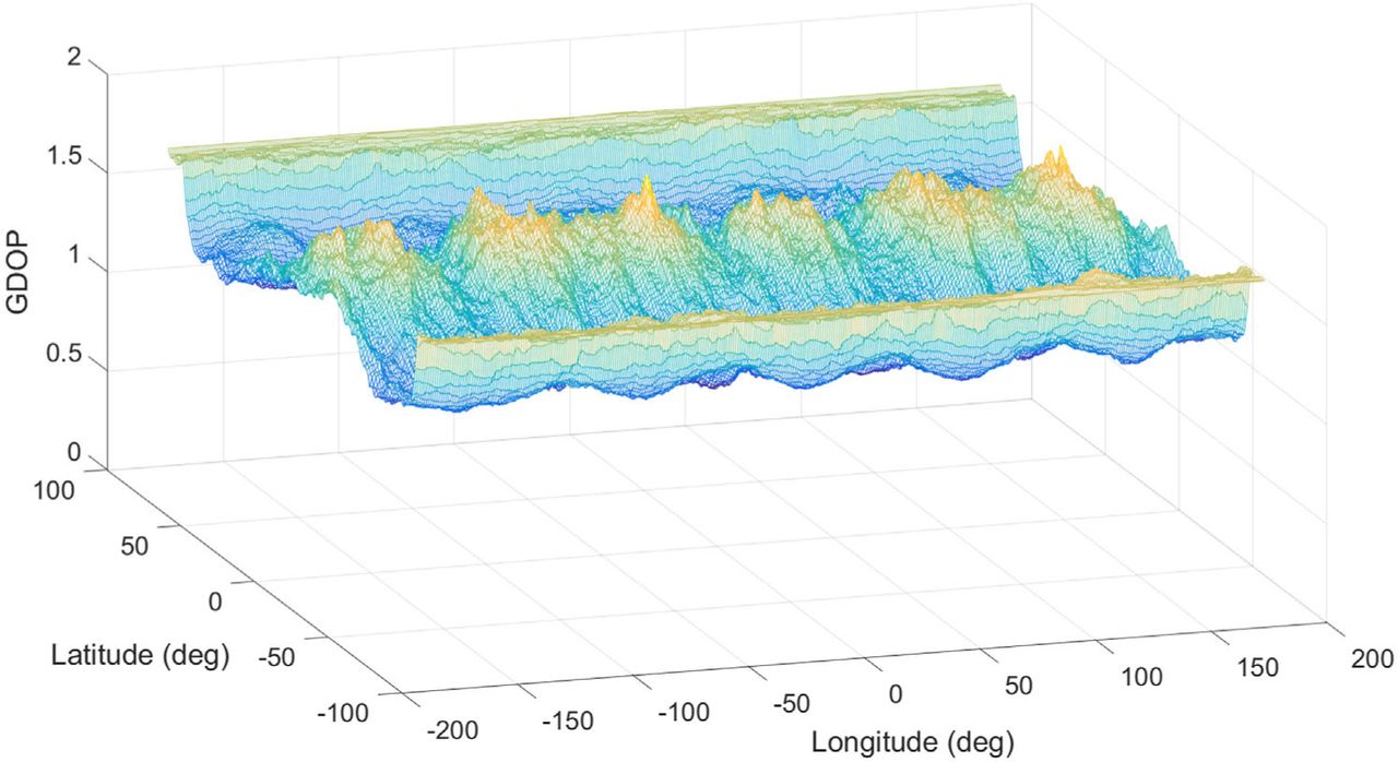
GDOP latitude/longitude map for 2825-satellite final Starlink constellation (𝛾𝑎𝑣𝑔 = 0.006 rad/sec, 𝜂𝑎𝑣𝑔 = 37 m/sec2)

Minimum and maximum GDOP vs. latitude for 2825-satellite final Starlink constellation (𝛾𝑎𝑣𝑔 = 0.006 rad/sec, 𝜂𝑎𝑣𝑔 = 37 m/sec2)
The value 𝜂𝑎𝑣𝑔 = 37 m/sec2 implies a clock offset precision of better than 2(0.01/37) = 0.00054 sec. These numbers are consistent with the batch filter results when operating on truth-model simulation data. This good GDOP map and relatively large values of 𝛾𝑎𝑣𝑔 and 𝜂𝑎𝑣𝑔 are the reasons why the final Starlink constellation has been chosen for purposes of evaluating the performance of the batch filter’s point solutions.
Note that the value of 𝛾𝑎𝑣𝑔 for this case is roughly six times larger than the average mean orbital motion  , which equals approximately 0.001 rad/sec. Similarly, the value of 𝜂𝑎𝑣𝑔 is more than five times larger than the acceleration of gravity at the satellites
  , which equals approximately 7 m/sec2. These amplification factors of six and five arise from the leading geometric terms in Equations (24) and (25), the ones that depend on the ratio 𝑅𝐸/𝑎𝑜𝑟𝑏. These high amplification factors are the result of using a LEO constellation. They are needed in order to obtain good performance from this system.
The GDOP minima and maxima vs. latitude for the initial Starlink constellation are shown in Figure 4. They are significantly different from those of the final constellation. The lack of high inclination orbits causes a sudden rise in GDOP above +50 degree latitude and below −50 degree latitude. This degradation happens even though there are 56 or more visible satellites at all longitudes around the globe for any latitude in the plotted range from −65 degree to +65 degree. This result illustrates the importance of proper geometric diversity of the directions of the  direction rate vectors. At high latitudes, all of the visible satellites have
  vectors that point nearly East for this constellation. The Kuiper constellation listed in Table 1 has similarly high GDOP values above +50 degree latitude and below −50 degree latitude.
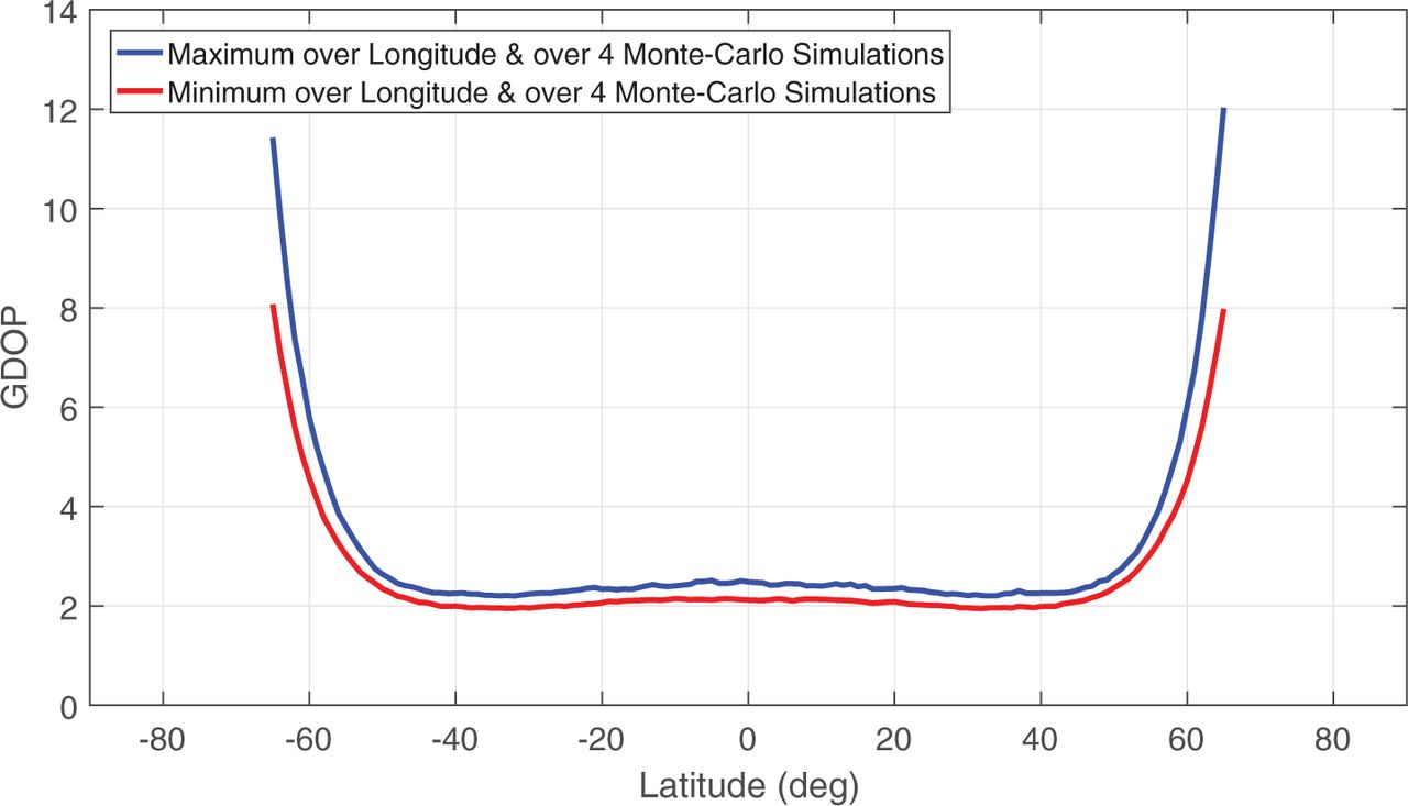
GDOP minima and maxima vs. latitude for 1600-satellite initial Starlink constellation (𝛾𝑎𝑣𝑔 = 0.006 rad/sec, 𝜂𝑎𝑣𝑔 = 39 m/sec2)
The importance of the geometric diversity of the directions of the  vectors is further illustrated by Figure 5’s GDOP map for the initial OneWeb constellation. This particular case assumes that all 18 ascending nodes of OneWeb’s nearly polar orbits are grouped together on one side of the Earth with 10 degree right ascension spacings between them. All 18 descending nodes are grouped together on the other side of the Earth. This configuration results in very high GDOP values near the equator and at mid latitudes whenever a given point on the Earth is visible only to North-going satellites or only to South-going satellites.

GDOP latitude/longitude map for 720-satellite initial OneWeb constellation with ascending nodes grouped together (𝛾𝑎𝑣𝑔 = 0.006 rad/sec, 𝜂𝑎𝑣𝑔 = 37 m/sec2)
Note the longitude regions of high GDOP between −180 degrees and −70 degrees, between −35 degrees and +110 degrees, and between +145 degrees and +180 degrees. This map shows low GDOP values near the equator and at mid latitudes along the two seams between the North-going and South-going clusters, i.e., in the longitude regions from −70 degrees to −35 degrees and from +110 degrees to +145 degrees. These are regions that have good geometric diversity of the  vectors’ directions.
The foregoing analysis of the poor OneWeb GDOP map of Figure 5 suggests a solution: Alternate the ascending and descending nodes of the orbital planes every other 10 degrees of right ascension. This alternate OneWeb constellation design has been analyzed to produce the GDOP minima and maxima vs. latitude shown in Figure 6.
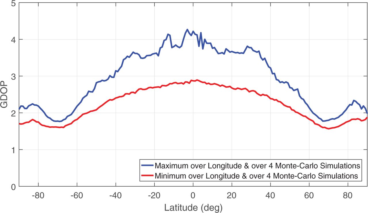
GDOP minima and maxima vs. latitude for 720-satellite initial OneWeb constellation with alternating ascending and descending nodes (𝛾𝑎𝑣𝑔 = 0.006 rad/sec, 𝜂𝑎𝑣𝑔 = 37 m/sec2)
This revised constellation’s maximum GDOP value is below 4.3, which is smaller than the maximum GDOP of Figure 5 by a factor of 23. This result confirms the importance of having a diversity of directions of the ̇ ̂ 𝜌𝑗 direction rate vectors.
Two important points have been illustrated by these GDOP studies: First, some of the planned large LEO constellations have a sufficient number of satellites with a sufficient diversity of orbits to enable accurate operation of the proposed system over the entire globe. Second, the ability to achieve good performance can be sensitive to constellation design parameters, (e.g., the distribution of the right ascensions of the ascending nodes and the upper limits of the orbital inclinations). Therefore, these types of GDOP mapping analyses should be performed for any constellation that is in serious contention for implementing this proposed system.
8 ADDITIONAL CONSIDERATIONS
A number of additional important issues must be addressed in order to make the proposed concept work in practice. This section introduces several of them.
8.1 Limited downlink signal footprint of each satellite
A significant concern about the constellations as presently configured has to do with downlink antenna gain patterns. These constellations are communication systems. It does not make sense for neighboring satellites to have large overlaps in their downlink coverage areas. Large overlaps would waste transmission power and would cause unneeded challenges to the problem of servicing multiple independent data transmission requests within the system’s limited spectrum.
The specific beam patterns and overlap possibilities vary for different constellations. One constant among all the constellations is the following: It is unlikely that any one user will see strong main-lobe downlink signals simultaneously from eight or more satellites of a given constellation.
Therefore, the system envisioned will be impossible to implement without some additional strategies to see enough satellites. One strategy might be to receive signals from downlink antenna side lobes. Given the high data rates envisioned by these systems, the main lobes will have a lot of power. Therefore, the side lobes may have sufficient power to enable signal acquisition and determination of carrier Doppler shift.
In this case, however, it will likely be necessary to know a given signal’s modulated bit pattern, at least for short bursts of data. The modulated pattern would be used as a pseudo PRN code and would allow a long enough coherent accumulation interval to enable signal acquisition and determination of carrier Doppler shift.
A second strategy could be to accept the limitation of seeing few satellites simultaneously and try to see enough different satellites over a short time window to get a good navigation fix. The use of an INS might help to navigate using a time series of carrier Doppler shift data. This concept has been studied in (McLemore & Psiaki, 2020) and shows promise.
A third strategy could be to modify a constellation’s satellites to carry special navigation beacon antennas with wide gain patterns. It would be allowable to put the beacon signals in a different frequency band than the given satellite’s communication signals. Each satellite could broadcast a narrowband beacon signal because there would be no need for a wideband ranging code. It might be allowable to broadcast a beacon signal intermittently with a short duty cycle, perhaps one 0.1 sec burst every second.
8.2 High frequencies of downlink signals
Current plans for these large constellations call for downlink signal frequencies in the range 11 GHz–40 GHz. Signals at these frequencies can experience significant attenuation by foliage and significant scattering by rain. It would be better to have signals in a lower frequency range. If a constellation owner decided to add a beacon signal with a wide-gain-pattern antenna, it would be best if that signal were at a significantly lower frequency than the currently planned downlink communication signals.
8.3 Additional error sources
The present study has not considered the degradation of accuracy that might be caused by multipath errors. A thorough analysis of the impact of multipath on carrier-Doppler-shift-based navigation should be carried out for this concept. Given the good performance that the author has experienced with velocity estimation based on GPS carrier Doppler shift measurements, there is reason to believe that the impacts of multipath will not be too deleterious, but the issue needs study.
A great amount of research has been carried out on the subject of multipath-induced errors, but almost all of it considers the effects on pseudorange and beat carrier phase. Xu and Rife (2019) is the only work known to this author that specifically considers multipath effects on carrier Doppler shift. Its methods and results are not directly applicable to the question of how multipath would affect the present system. Therefore, a new type of multipath study will be needed to address this issue.
Another potential source of accuracy degradation is the mismatch between the true troposphere and ionosphere effects on carrier Doppler shift and the models for these effects that will be used by the batch filter. There is reason to hope that the impact of atmospheric mis-modeling will be small. Again, this hope comes from the good results for velocity estimation from carrier Doppler shift that have been achieved when completely ignoring atmospheric effects. Nevertheless, this issue must be carefully studied.
Most studies of troposphere and ionosphere effects consider only pseudorange and beat carrier phase. Graziani et al. (2009) examines a method for estimating and correcting troposphere effects of carrier Doppler shift measurements from deep space probes. (Klobuchar, 1996) briefly discusses ionosphere effects on carrier Doppler shift. However, neither of these works analyze the effects of troposphere or ionosphere modeling errors in a way that is directly relevant to the present system. To this author’s knowledge, no other published works address these questions in ways that would be relevant to this study. Therefore, research on these topics must develop new methods to address these concerns.
8.4 Signal design and signal processing for multiple access operation
The necessity to distinguish signals from 2,000 or more satellites, perhaps with 100 or more of them arriving simultaneously, raises issues of multiple access. If the satellites are to carry special beacons, then a way must be found to design signals so that they can all fit into a relatively narrow bandwidth and yet all be distinguishable. Therefore, effective multiple access strategies will be needed. The possibilities of code-division, frequency division, and time-division multiple access could be considered. Signal processing strategies for such multiple access signals would have to be developed in tandem with their signal structures.
If the existing signals are to be used, including side-lobe signals, then ways will have to be devised to distinguish among the many side-lobe signals that will be present in weak form. It is not clear whether this will be feasible. This problem is worth considering for the following reason: If it can be solved, then this navigation concept might be able to use a constellation such as OneWeb without requiring hardware modifications.
A solution to the side-lobe problem might involve sending special short data messages on the constellation’s downlinks that serve as PRN codes to enable multiple access and long coherent integration of weak side-lobe signals. If the constellation did not cooperate by broadcasting the needed data messages, then it might be possible to listen to main-lobe signals from a network of ground stations and provide after-the-fact information about modulated data. Such a system, however, would require a means to disseminate information about modulated data, which would involve high-bandwidth data broadcasts to user receivers. It would also introduce latency to their navigation solutions.
8.5 Batch filter convergence from large initial errors
The point-solution batch filter has been tested for its convergence capability from initial horizontal errors on the order of 150 km. A cold start capability would require assured convergence to the optimal solution from a first guess that is much farther away from the true position than 150 km. There likely exist good ways to ensure a large region of convergence of the batch filter, but additional work may need to be done to devise and implement a suitable strategy for ensured convergence.
8.6 Use of signals from multiple constellations
This study has considered signals that all come from one or the other of the several constellations that are being planned or fielded. It might make sense to use signals from multiple constellations. Such an approach could alleviate some of the GDOP problems that have been noted in the previous section.
McLemore and Psiaki (2020) have already considered this issue to a limited extent. Their proceeding paper examines possible use of the Iridium constellation in conjunction with either OneWeb, Starlink, or Kuiper. In a multi-constellation approach, it is not necessary that any one of the constituent constellations be able to provide full 4D navigation. Thus, the use of the existing Iridium constellation is reasonable within a multi-constellation system.
The usefulness of multiple constellations hinges on various factors such as signal ground footprints, the resulting impact on GDOP, and the practicality of designing and building receivers to cover the various frequency bands used by the constellations. These issues should all be studied in hopes of finding a multi-constellation solution that is practical.
8.7 Determining accurate satellite ephemerides and clock frequency offsets independent of existing GNSS
The present study has considered the impact of satellite ephemeris and clock frequency errors on navigation solution accuracy. The levels of errors considered, 2 m RMS per-axis position error, 0.002 m/sec RMS per-axis velocity error, and 3.3× 10⁻¹¹ seconds/sec clock frequency error, may be challenging to achieve for a stand-alone system that uses neither onboard GNSS receivers nor onboard atomic clocks.
Some sort of ground-control segment would have to be set up. It would operate a global network of receivers at accurately surveyed locations that have very stable clocks. They could estimate orbits and satellite transmitter clock frequency offsets based on the same carrier Doppler shift signals that support user equipment navigation. Such a system may be able to achieve the stated levels of accuracy if designed properly. The nearest existing equivalent based on on-way carrier Doppler shift is the DORIS orbit determination system (Jayles & Costes, 2004).
This study provides hope that the accuracies stated above might be achievable within a period when data are available. Whether they could be achieved over a needed forward prediction interval is an open question. The largest challenge might be clock frequency prediction.
It might be possible to address this challenge using constellation cross-links, if available, to distribute a frequency standard to the entire constellation that originates from radio-frequency links between a few satellites and a small number of ground stations. An alternative approach might be to link each satellite to a ground station often. Such an approach would reduce the needed prediction interval for clock frequency, but it would require a large network of ground stations.
It may be possible to achieve good user navigation accuracy with less accuracy of the ephemerides and transmitter clock frequencies than has been assumed in this paper. Perhaps the user equipment filter could consider states to allow for ephemeris and transmitter clock frequency errors.
The achievable accuracies of the ephemerides and the transmitter clock frequency offsets for an independent system and their impact on navigation error are worthy subjects for future research. These will be very important topics if independence from MEO GNSS is a requirement of such a system.
9 SUMMARY AND CONCLUSIONS
A new Global Navigation Satellite System (GNSS) has been proposed. It uses carrier Doppler shift as its only observable. It exploits the simultaneous visibility of eight or more satellites that will be a hallmark of the large Low Earth Orbit (LEO) constellations that are being planned and fielded. The availability of carrier Doppler shift measurements from eight or more satellites makes 3D position, receiver clock offset, 3D velocity, and receiver clock offset rate simultaneously observable. These quantities can be estimated by using a new type of point solution that replaces the pseudorange equations of traditional GNSS with carrier Doppler shift equations.
A new Geometric Dilution of Precision (GDOP) analysis has been developed for this concept. It reaffirms the importance of the geometric diversity of the Line-of-Sight (LOS) unit direction vectors from the visible satellites to the receiver, as in pseudorange-based GNSS, but it brings to light additional important factors: The magnitudes and the geometric diversity of the rates of change of the LOS direction vectors are important to achieving low GDOP. The magnitudes of the range accelerations between the satellites and the receiver are also important to achieving low GDOP. These factors dictate that the satellites be in LEO and that the visible satellites at any given point on the Earth have a diversity of velocities relative to the receiver. Proper constellation design can ensure that all of the requirements for low GDOP are met.
Batch filter results for truth-model simulation data and GDOP studies both indicate that absolute position accuracies on the order of 1 meter to 5 meters and absolute velocity accuracies on the order of 0.01 m/sec to 0.05 m/sec may be achievable for a system with carrier Doppler shifts that can be measured with an equivalent range-rate accuracy of 0.01 m/sec 1-𝜎.
The only weak part of this system is its timing accuracy. Errors on the order of 0.0002 to 0.0004 sec 1-𝜎 are likely. Nevertheless, time is absolutely observable with this system, and it does not require that the LEO constellation carry atomic clocks or transmit ranging codes.
Additional work will be required in order to realize such a system using planned constellations and signals. The encouraging possibilities analyzed in this study provide a motivation for doing the needed work.
HOW TO CITE THIS ARTICLE
Psiaki ML. Navigation using carrier Doppler shift from a LEO constellation: TRANSIT on steroids. NAVIGATION. 2021;68:621–641. https://doi.org/10.1002/navi.438
AUTHOR BIOGRAPHY
Mark L. Psiaki is Professor and Kevin T. Crofton Faculty Chair of Aerospace and Ocean Engineering at Virginia Tech. He is also Professor Emeritus of Mechanical and Aerospace Engineering at Cornell University. He holds a Ph.D. in Mechanical and Aerospace Engineering from Princeton University. He is a Fellow of both the ION and the AIAA. His research interests are in the areas of navigation, spacecraft attitude and orbit determination, remote sensing, and general methods for estimation, filtering, and detection.
APPENDIX A: DERIVATION OF ANALYTIC CARRIER DOPPLER SHIFT MODEL
This appendix derives the analytic carrier Doppler shift model in Equation (7) starting from Equations (1)-(6). The derivation starts by substituting Equation (3) into Equation (1) while applying the chain rule in order to transform from differentiation with respect to true reception time 𝑇𝑅 to differentiation with respect to erroneous receiver clock time 𝑡𝑅. The time derivatives of the neutral atmosphere term  and the ionosphere term
  are neglected, in keeping with the stated assumptions of Equation (7). The result for the 𝑗th satellite’s signal is:
 A1
A1
where:
 A2
A2
is the range from the satellite to the receiver. Time differentiation of this range expression with respect to 𝑇𝑅 yields:
 A3
A3
The first term on the right-hand side of this equation accounts for the direct dependence of  and
and  on 𝑇𝑅 = 𝑡𝑅 −𝛿𝑅. The second term accounts for the dependence of
  and
and  on
on  , which depends on 𝑇𝑅. Time differentiation of Equation (4) with respect to 𝑇𝑅 and neglect of the time derivatives of the neutral atmosphere and ionosphere terms yields a second equation involving 𝑑𝜌𝑗/𝑑𝑇𝑅 and
  :
:
 A4
A4
Simultaneous solution of Equations (A3) and (A4) for their two unknowns yields:
 A5
A5
The only remaining unknown in Equation (A1) is 𝑑𝑇𝑅/𝑑𝑡𝑅. It can be determined by differentiating the known relationship 𝑇𝑅 = 𝑡𝑅 −𝛿𝑅 with respect to 𝑇𝑅, solving for 𝑑𝑡𝑅/𝑑𝑇𝑅, and taking the reciprocal of the result. This process yields:
 A6
A6
Equations (A1), (A5), and (A6) can be combined to yield the formula in Equation (7). This procedure substitutes the 𝑑𝜌𝑗/𝑑𝑇𝑅 and  formulas from Equation (A5) and the 𝑑𝑇𝑅/𝑑𝑡𝑅 formula from Equation (A6) into the right-hand side of Equation (A1). Afterward, both sides of the resulting equation are multiplied by −𝜆, and several algebraic rearrangements are performed to yield the formula in Equation (7).
- Received October 16, 2020.
- Revision received June 20, 2021.
- Accepted July 5, 2021.
- © 2021 Institute of Navigation
This is an open access article under the terms of the Creative Commons Attribution License, which permits use, distribution and reproduction in any medium, provided the original work is properly cited.


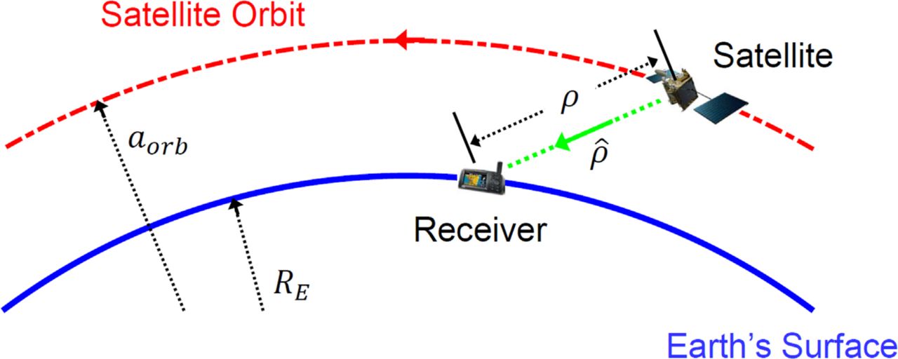
Jump to section
- Article
- Abstract
- 1 INTRODUCTION
- 2 CARRIER DOPPLER SHIFT MEASUREMENT MODELS
- 3 REVIEW OF LARGE LEO CONSTELLATIONS AND THEIR SUITABILITY FOR DOPPLER-ONLY PNT
- 4 POINT SOLUTIONS USING A BATCH LEAST-SQUARES FILTER
- 5 POINT-SOLUTION BATCH FILTER PERFORMANCE ON EXAMPLE SIMULATED DATA
- 6 A GENERALIZED GDOP ANALYSIS FOR DOPPLER-ONLY PNT
- 7 GDOP-BASED CONSTELLATION ANALYSES
- 8 ADDITIONAL CONSIDERATIONS
- 9 SUMMARY AND CONCLUSIONS
- HOW TO CITE THIS ARTICLE
- AUTHOR BIOGRAPHY
- APPENDIX A: DERIVATION OF ANALYTIC CARRIER DOPPLER SHIFT MODEL
- REFERENCES
- Figures & Data
- Supplemental
- References
- Info & Metrics
Related Articles
Cited By...
- No citing articles found.