

Abstract
Reliably assessing the error in an estimated vehicle position is integral for ensuring the vehicle’s safety in urban environments. Many existing approaches use GNSS measurements to characterize protection levels (PLs) as probabilistic upper bounds on position error. However, GNSS signals might be reflected or blocked in urban environments, and thus additional sensor modalities need to be considered to determine PLs. In this paper, we propose an approach for computing PLs by matching camera image measurements to a LiDAR-based 3D map of the environment. We specify a Gaussian mixture model probability distribution of position error using deep neural-network-based data-driven models and statistical outlier weighting techniques. From the probability distribution, we compute PL by evaluating the position error bound using numerical line-search methods. Through experimental validation with real-world data, we demonstrate that the PLs computed from our method are reliable bounds on the position error in urban environments.
- deep learning
- image registration
- integrity monitoring
- localization safety
- protection level
- vision-based localization
1 INTRODUCTION
In recent years, research on autonomous navigation for urban environments has been garnering increasing attention. Many publications have targeted different aspects of navigation such as route planning (Delling et al., 2017), perception (Jensen et al., 2016), and localization (Caselitz et al., 2016; Wolcott & Eustice, 2017). For trustworthy operation in each of these aspects, assessing the level of safety of the vehicle from potential system failures is critical. However, few works have examined the problem of safety quantification for autonomous vehicles.
In the context of satellite-based localization, safety is typically addressed via integrity monitoring (IM) (Spilker Jr. et al., 1996). Within IM, protection levels (PLs) specify a statistical upper bound on the error in an estimated position of the vehicle, which can be trusted to enclose the position errors with a required probabilistic guarantee. To detect an unsafe estimated vehicle position, these protection levels are compared with the maximum allowable position error value, known as the alarm limit.
Various methods (Cezón et al., 2013; Jiang & Wang, 2016; Tran & Lo Presti, 2019) have been proposed over the years for computing protection levels, however, most of these approaches focus on GNSS-only navigation. These approaches do not directly apply to GNSS-denied urban environments, where visual sensors are becoming increasingly preferred (Badue et al., 2021). Although various options in visual sensors exist in the market, camera sensors are inexpensive, lightweight, and have been widely employed in industry. For quantifying localization safety in GNSS-denied urban environments, there is thus a need to develop new ways of computing protection levels using camera image measurements.
Since protection levels are bounds over position error, computing them from camera image measurements requires a model that relates the measurements to position error in the estimate of the vehicle location. Furthermore, since the lateral, longitudinal, and vertical directions are well-defined with respect to a vehicle’s location on the road, the model must estimate the maximum position error in each of these directions for computing protection levels (Reid et al., 2019). However, characterizing such a model is not so straightforward. This is because the relation between a vehicle location in an environment and the corresponding camera image measurement is complex, depending on identifying and matching structural patterns in the measurements with prior known information about the environment (Caselitz et al., 2016; Kim et al., 2018; Taira et al., 2021; Wolcott & Eustice, 2017).
Recently, data-driven techniques based on deep neural networks (DNN) have demonstrated state-of-the-art performance in determining the state of the camera sensor, comprised of its position and orientation, by identifying and matching patterns in images with a known map of the environment (Cattaneo et al., 2019; Lyrio et al., 2015; Oliveira et al., 2020) or an existing database of images (Sarlin et al., 2019; Taira et al., 2021).
By leveraging data sets consisting of multiple images with known camera states in an environment, these approaches can train a DNN to model the relationship between an image and the corresponding state. However, the model characterized by the DNN can often be erroneous or brittle. For instance, recent research has shown that the output of a DNN can change significantly with minimal changes to the inputs (Recht et al., 2019). Thus, for using DNNs to determine position error, uncertainty in the output of the DNN must also be addressed.
DNN-based algorithms consider two types of uncertainty (Kendall & Gal, 2017; Loquercio et al., 2020). Aleatoric or statistical uncertainty results from the noise present in the inputs to the DNN, because of which a precise output cannot be produced. For camera image inputs, sources of noise include illumination changes, occlusion, or the presence of visually ambiguous structures, such as windows tessellated along a wall (Kendall & Gal, 2017). On the other hand, epistemic or systematic uncertainty exists within the model itself. Sources of epistemic uncertainty include poorly determined DNN model parameters as well as external factors that are not considered in the model (Kiureghian & Ditlevsen, 2009), such as environmental features which might be ignored by the algorithm while matching the camera images to the environment map.
While aleatoric uncertainty is typically modeled as the input-dependent variance in the output of the DNN (Kendall & Gal, 2017; McAllister et al., 2017; Yang et al., 2020), epistemic uncertainty relates to the DNN model and, therefore, requires further deliberation. Existing approaches approximate epistemic uncertainty by assuming a probability distribution over the weight parameters of the DNN to represent ignorance about the correct parameters (Blundell et al., 2015; Gal & Ghahramani, 2016; Kendall & Cipolla, 2016).
However, these approaches assume that a correct value of the parameters exists and that the probability distribution over the weight parameters captures the uncertainty in the model, both of which do not necessarily hold up in practice (Smith & Gal, 2018). This inability of existing DNN-based methods to properly characterize uncertainty limits their applicability to safety-critical applications, such as the localization of autonomous vehicles.
In this paper, we propose a novel method for computing protection levels associated with a given vehicular state estimate (position and orientation) from camera image measurements and a 3D map of the environment. This work is based on our recent ION GNSS+ 2020 conference paper (Gupta & Gao, 2020) and includes additional experiments and improvements to the DNN training process.
Recently, high-definition 3D environment maps in the form of LiDAR point clouds have become increasingly available through industry players such as HERE, TomTom, Waymo, and NVIDIA, as well as through projects such as USGS 3DEP (Lukas & Stoker, 2016) and OpenTopography (Krishnan et al., 2011). Furthermore, LiDAR-based 3D maps are more robust to noise from environmental factors, such as illumination and weather, than image-based maps (Wang et al., 2020). Hence, we use LiDAR-based 3D point cloud maps in our approach.
Previously, CMRNet (Cattaneo et al., 2019) has been proposed as a DNN-based approach for determining the vehicular state from camera images and a LiDAR-based 3D map. In our approach, we extend the DNN architecture proposed in Cattaneo et al. (2019) to model the position error and the covariance matrix (aleatoric uncertainty) in the vehicular state estimate.
To assess the epistemic uncertainty in position error, we evaluate the DNN position error outputs at multiple candidate states in the vicinity of the state estimate, and combine the outputs into samples of the state estimate position error. Figure 1 shows the architecture of our proposed approach.
Given a state estimate, we first select multiple candidate states from its neighborhood. Using the DNN, we then evaluate the position error and covariance for each candidate state by comparing the camera image measurement with a local map constructed from the candidate state and 3D environment map. Next, we linearly transform the position error and covariance outputs from the DNN with relative positions of candidate states into samples of the state estimate position error and variance. We then separate these samples into the lateral, longitudinal, and vertical directions and weight the samples to mitigate the impact of outliers in each direction. Subsequently, we combine the position error samples, outlier weights, and variance samples to construct a Gaussian mixture model probability distribution of the position error in each direction, and numerically evaluate its intervals to compute protection levels.

Architecture of our proposed approach for computing protection levels. Given a state estimate, multiple candidate states are selected from its neighborhood and the corresponding position error and the covariance matrix for each candidate state are evaluated using the DNN. The position errors and covariance are then linearly transformed to obtain samples of the state estimate position error and variance, which are then weighted to determine outliers. Finally, the position error samples, outlier weights, and variance are combined to construct a Gaussian mixture model probability distribution, from which the lateral, longitudinal, and vertical protection levels are computed through numerical evaluation of its probability intervals
Our main contributions are as follows:
We extend the CMRNet (Cattaneo et al., 2019) architecture to model both the position error in the vehicular state estimate and the associated covariance matrix. Using the 3D LiDAR-based map of the environment, we first construct a local map representation with respect to the vehicular state estimate. Then, we use the DNN to analyze correspondence between the camera image measurement and the local map for determining the position error and the covariance matrix
We develop a novel method for capturing epistemic uncertainty in the DNN position error output. Unlike existing approaches which assume a probability distribution over DNN weight parameters, we directly analyze different position errors that are determined by the DNN for multiple candidate states selected from within a neighborhood of the state estimate. The position error outputs from the DNN corresponding to the candidate states are then linearly combined with the candidate states’ relative position from the state estimate to obtain an empirical distribution of the state estimate position error
We design an outlier weighting scheme to account for possible errors in the DNN output at inputs that differ from the training data. Our approach weighs the position error samples from the empirical distribution using a robust outlier detection metric known as a robust Z-score (Iglewicz & Hoaglin, 1993), along the lateral, longitudinal, and vertical directions individually
We construct the lateral, longitudinal, and vertical protection levels as intervals over the probability distribution of the position error. We model this probability distribution as a Gaussian mixture model (Lindsay, 1995) from the position error samples, DNN covariance, and outlier weights
We demonstrate the applicability of our approach in urban environments by experimentally validating the protection levels computed from our method using real-world data with multiple camera images and different state estimates
The remainder of this paper is structured as follows: Section 2 discusses related work; Section 3 formulates the problem of estimating protection levels; Section 4 describes the two types of uncertainties considered in our approach; Section 5 details our algorithm; Section 6 presents the results from experimentation with real-world data; and we conclude the paper in Section 7.
2 RELATED WORK
Several methods have been developed over the years which characterize protection levels in the context of GNSS-based urban navigation. Jiang and Wang (2016) computed horizontal protection levels using an iterative search-based method and test statistic based on the bivariate normal distribution. Cezón et al. (2013) analyzed methods which utilize the isotropy of residual vectors from the least-squares position estimation to compute the protection levels. Tran and Lo Presti (2019) combined advanced receiver autonomous integrity monitoring (ARAIM) with Kalman filtering, and computed the protection levels by considering the set of position solutions which arise after excluding faulty measurements.
These approaches compute the protection levels by deriving the mathematical relation between measurement and position domain errors. However, such a relation is difficult to formulate with camera image measurements and a LiDAR-based 3D map, since the position error in this case depends on various factors such as the structure of buildings in the environment, available visual features, and illumination levels.
Previous works have proposed IM approaches for LiDAR- and camera-based navigation where the vehicle is localized by associating identified landmarks with a stored map or a database. Joerger and Pervan (2019) developed a method to quantify integrity risk for LiDAR-based navigation algorithms by analyzing failures of feature extraction and data association subroutines. Zhu et al. (2020) derived a bound on the integrity risk in camera-based navigation using EKF caused by incorrect feature associations.
However, these IM approaches have been developed for localization algorithms based on data association and cannot be directly applied to many recent camera and LiDAR-based localization techniques which use deep learning to model the complex relation between measurements and the stored map or database. Furthermore, these IM techniques do not estimate protection levels, which are the focus of our work.
Deep learning has been widely applied to determine position information from camera images. Kendall et al. (2015) trained a DNN using images from a single environment to learn the relationship between image and the camera 6-DOF pose. Taira et al. (2021) learned image features using a DNN to apply feature extraction and matching techniques to estimate the 6-DOF camera pose relative to a known 3D map of the environment. Sarlin et al. (2019) developed a deep learning-based 2D-3D matching technique to obtain a 6-DOF camera pose from images and a 3D environment model. However, these approaches do not model the corresponding uncertainty associated with the estimated camera pose, or account for failures in DNN approximation (Smith & Gal, 2018), which is necessary for characterizing safety measures such as protection levels.
Some recent works have proposed to estimate the uncertainty associated with deep learning algorithms. Kendall and Cipolla (2016) estimate the uncertainty in DNN-based camera pose estimation from images by evaluating the network multiple times through dropout (Gal & Ghahramani, 2016). Loquercio et al. (2020) propose a general framework for estimating uncertainty in deep learning as variance computed from both aleatoric and epistemic sources. McAllister et al. (2017) suggest using Bayesian deep learning to determine uncertainty and quantify safety in autonomous vehicles by placing probability distributions over DNN weights to represent the uncertainty in the DNN model. Yang et al. (2020) jointly estimate the vehicle odometry, scene depth, and uncertainty from sequential camera images.
However, the uncertainty estimates from these algorithms do not take into account the inaccuracy of the trained DNN model, or the influence of the underlying environment structure on the DNN outputs. In our approach, we evaluate the DNN position error outputs at inputs corresponding to multiple states in the environment, and utilize these position errors for characterizing uncertainty both from inaccuracy in the DNN model as well as from the environment structure around the state estimate.
To the best of our knowledge, our approach is the first that applies data-driven algorithms for computing protection levels by characterizing the uncertainty from different error sources. The proposed method seeks to leverage the high-fidelity function modeling capability of DNNs and combine it with techniques from robust statistics and integrity monitoring to compute robust protection levels using camera image measurements and 3D maps of the environment.
3 PROBLEM FORMULATION
Consider the scenario of a vehicle navigating in an urban environment using measurements acquired by an onboard camera. The 3D LiDAR map of the environment ℳ that consists of points p ∈ ℝ3 is assumed to be pre-known from either openly available repositories (Krishnan et al., 2011; Lukas & Stoker, 2016) or simultaneous localization and mapping algorithms (Cadena et al., 2016).
The vehicular state st = [xt, ot] at time t is a seven-element vector comprising of its 3D position xt = [xt,yt,zt]T ∈ ℝ3 along x, y, and z dimensions as well as 3D orientation unit quaternion ot = [o1,t,o2,t,o3,t,o4,t] ∈ SU(2). The vehicle state estimates over time are denoted as  where Tmax denotes the total time in a navigation sequence. At each time t, the vehicle captures an RGB camera image It ∈ ℝl × w × 3 from the onboard camera where l and w denote pixels along length and width dimensions, respectively.
Given an integrity risk specification IR, our objective is to compute the lateral protection level PLlat,t, longitudinal protection level PLlon,t, and vertical protection level PLvert,t at time t, which denote the maximal bounds on the position error magnitude with a probabilistic guarantee of at least 1 − IR. Considering x, y, and z dimensions in the rotational frame of the vehicle:
 1
1
where  denotes the unknown true vehicle position at time t.
4 TYPES OF UNCERTAINTY IN POSITION ERROR
Protection levels for a state estimate st at time t depend on the uncertainty in determining the associated position error Δxt = [Δxt,Δyt,Δzt] between the state estimate position xt and the true position  from the camera image It and the environment map ℳ. We consider two different kinds of uncertainty, which are categorized by the source of inaccuracy in determining the position error Δxt: aleatoric uncertainty and epistemic uncertainty.
4.1 Aleatoric uncertainty
Aleatoric uncertainty refers to the uncertainty from noise present in the camera image measurements It and the environment map ℳ, due to which a precise value of the position error Δxt cannot be determined. Existing DNN-based localization approaches model the aleatoric uncertainty as a covariance matrix with only diagonal entries (Kendall & Gal, 2017; McAllister et al., 2017; Yang et al., 2020) or with both diagonal and off-diagonal terms (Liu et al., 2018; Russell & Reale, 2019).
Similar to the existing approaches, we characterize the aleatoric uncertainty by using a DNN to model the covariance matrix Σt associated with the position error Δxt. We consider both nonzero diagonal and off-diagonal terms in Σt to model the correlation between x-, y-, and z-dimension uncertainties, such as along the ground plane.
Aleatoric uncertainty by itself does not accurately represent the uncertainty in determining position error. This is because aleatoric uncertainty assumes that the noise present in training data also represents the noise in all future inputs and the DNN approximation is error-free. These assumptions fail in scenarios when the input at evaluation time is different from the training data or when the input contains features that occur rarely in the real world (Smith & Gal, 2018). Thus, relying purely on aleatoric uncertainty can lead to overconfident estimates of the position error uncertainty (Kendall & Gal, 2017).
4.2 Epistemic uncertainty
Epistemic uncertainty relates to the inaccuracies in the model for determining the position error Δxt. In our approach, we characterize the epistemic uncertainty by leveraging a geometrical property of the position error Δxt, where for the same camera image It, Δxt can be obtained by linearly combining the position error  computed for any candidate state
  and the relative position of
  from the state estimate st (Figure 2). Hence, using known relative positions and orientations of NC candidate states
  from st, we transform the different position errors
  determined for the candidate states into samples of the state estimate position error Δxt. The empirical distribution comprised of these position error samples characterizes the epistemic uncertainty in the position error estimated using the DNN.
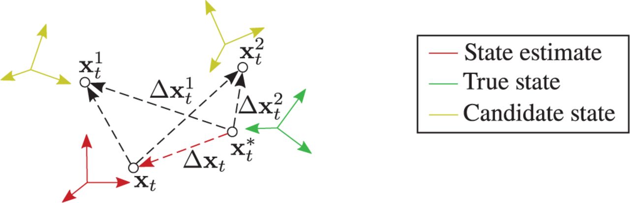
Position error Δxt in the state estimate position xt is a linear combination of the position error  in position
  of any candidate state
  and the relative position vector between
5 DATA-DRIVEN PROTECTION LEVELS
This section details our algorithm for computing data-driven protection levels for the state estimate st at time t, using the camera image It and environment map ℳ. First, we describe the method for generating local representations of the 3D environment map ℳ with respect to the state estimate st. Then, we illustrate the architecture of the DNN. Next, we discuss the loss functions used in DNN training. We then detail the method for selecting multiple candidate states from the neighborhood of the state estimate st.
Using the position errors and covariance matrix evaluated from the DNN for each of these candidate states, we then illustrate the process for transforming the candidate state position errors into multiple samples of the state estimate position error. To mitigate the impact of outliers on the computed position error samples in each of the lateral, longitudinal, and vertical directions, we then detail the procedure for computing outlier weights. Next, we characterize the probability distribution over position error in lateral, longitudinal, and vertical directions. Finally, we detail the approach for determining protection levels from the probability distribution by numerical methods.
5.1 Local map construction
A local representation of the 3D LiDAR map of the environment captures the environment information in the vicinity of the state estimate st at time t. By comparing the environment information captured in the local map with the camera image It ∈ ℝl × w × 3 using a DNN, we estimate the position error Δxt and covariance Σt in the state estimate st.
For computing local maps, we utilize the LiDAR-image generation procedure described in Cattaneo et al. (2019). Similar to their approach, we generate the local map L(s, ℳ) ∈ ℝl × w associated with vehicle state s and LiDAR environment map ℳ in two steps.
First, we determine the rigid-body transformation matrix Hs in the special Euclidean group SE(3) corresponding to the vehicle state s:
 2
2where
– Rs denotes the rotation matrix corresponding to the orientation quaternion elements o = [o1,o2,o3,o4] in the state s
– Ts denotes the translation vector corresponding to the position elements x = [x,y,z] in the state s
Using the matrix Hs, we rotate and translate the points in the map ℳ to the map ℳs in the reference frame of the state s:
3where I denotes the identity matrix. For maintaining computational efficiency in the case of large maps, we use the points in the LiDAR map ℳs that lie in a subregion around the state s and in the direction of the vehicle orientation.
In the second step, we apply the occlusion estimation filter presented in Pintus et al. (2011) to identify and remove occluded points along rays from the camera center. For each pair of points (p(i),p(j)) where p(i) is closer to the state s, p(j) is marked occluded if the angle between the ray from p(j) to the camera center and the line from p(j) to p(i) is less than the threshold. Then, the remaining points are projected to the camera image frame using the camera projection matrix K to generate the local depth map L(s, ℳ). The i-th point p(i) in ℳs is projected as:
4where
– px,py denote the projected 2D coordinates with scaling term c
– [L(s, ℳ)](px, py) denotes the (px,py) pixel position in the local map L(s, ℳ)


The local depth map L(s, ℳ) for state s visualizes the environment features that are expected to be captured in a camera image obtained from the state s. However, the obtained camera image It is associated with the true state  that might be different from the state estimate st. Nevertheless, for reasonably small position and orientation differences between the state estimate st and true state
  , the local map L(s, ℳ) contains features that correspond with some of the features in the camera image It that we use to estimate the position error.
5.2 DNN architecture
We use a DNN to estimate the position error Δxt and associated covariance matrix Σt by implicitly identifying and comparing the positions of corresponding features in camera image It and the local depth map L(st, ℳ) associated with the state estimate st.
The architecture of our DNN is given in Figure 3. Our DNN is comprised of two separate modules: one for estimating the position error Δxt and other for the parameters of the covariance matrix Σt. The first module for estimating the position error Δxt is based on CMRNet (Cattaneo et al., 2019).

Architecture of our deep neural network (DNN) for estimating translation and rotation errors as well as parameters of the covariance matrix. The translation and rotation errors are determined using CMRNet (Cattaneo et al., 2019), and employs correlation layers (Dosovitskiy et al., 2015) for comparing feature representations of the camera image and the local depth map. Using a similar architecture, we design CovarianceNet which produces parameters of the covariance matrix associated with the translation error output
CMRNet was originally proposed as an algorithm to iteratively determine the position and orientation of a vehicle using a camera image and 3D LiDAR map, starting from a provided initial state. For determining position error Δxt using CMRNet, we use the state estimate st as the provided initial state and the corresponding DNN translation  and rotation
  error output for transforming the state st towards the true state
  . Formally, given any state s and camera image It at time t, the translation error
  and rotation error
  are expressed as:
 5
5
CMRNet estimates the rotation error  as a unit quaternion. Furthermore, the architecture determines both the translation error
  and rotation error
  in the reference frame of the state s. Since the protection levels depend on the position error Δx in the reference frame from which the camera image It is captured (the vehicle reference frame), we transform the translation error
  to the vehicle reference frame by rotating it with the inverse of
  :
:
 6
6
where  is the 3 × 3 rotation matrix corresponding to the rotation error quaternion
  .
.
In the second module, we determine the covariance matrix Σ associated with Δx by first estimating the covariance matrix  associated with the translation error
  obtained from CMRNet and then transforming it to the vehicle reference frame using
  .
.
We model the covariance matrix  by following a similar approach to Russell & Reale (2019). Since the covariance matrix is both symmetric and positive-definite, we consider the decomposition of
  into diagonal standard deviations σ = [σ1,σ2,σ3] and correlation coefficients η = [η21,η31,η32]:
 7
7
where i, j ∈ {1, 2, 3} and j < i. We estimate these terms using our second DNN module (referred to as CovarianceNet) which has a similar network structure as CMR-Net, but with 256 and 6 artificial neurons in the last two fully connected layers to prevent overfitting.
For stable training, CovarianceNet produces a logarithm of the standard deviation output, which is converted to the standard deviation by then taking the exponent. Additionally, we use tanh function to scale the correlation coefficient outputs η in CovarianceNet between ±1. Formally, given a vehicle state s and camera image It at time t, while the standard deviation σ and correlation coefficients η is approximated as:
 8
8
Using the constructed  from the obtained σ, η, we obtain the covariance matrix Σ associated with Δx as:
 9
9
We keep the aleatoric uncertainty restricted to position domain errors in this work for simplicity, and thus treat  as a point estimate. The impact of errors in estimating
  on protection levels is taken into consideration as epistemic uncertainty and discussed in more detail in Sections 5.5 and 5.7.
The feature extraction modules in CovarianceNet and CMRNet are separate since the two tasks are complementary; for estimating position error, the DNN must learn features that are robust to noise in the inputs while the variance in the estimated position error depends on the noise itself.
5.3 Loss functions
The loss function for training the DNN must penalize position error outputs that differ from the corresponding ground truth present in the dataset, as well as penalize any covariance that overestimates or underestimates the uncertainty in the position error predictions. Furthermore, the loss must incentivize the DNN to extract useful features from the camera image and local map inputs for predicting the position error. Hence, we consider three additive components in our loss function  (·):
(·):
 10
10
where:
–
, denotes the vector-valued translation and rotation error in the reference frame of the state estimate s to the unknown true state s*–
Huber(·) denotes the Huber loss function (Huber, 1992)–
MLE(·) denotes the loss function for the maximum likelihood estimation of position error Δx and covariance –
Ang(·) denotes the quaternion angular distance from Cattaneo et al. (2019)– αHuber,αMLE,αAng are coefficients for weighting each loss term


We employ the Huber loss  Huber(·) and quaternion angular distance
  Ang(·) terms from Cattaneo et al. (2019). The Huber loss term
  Huber(·) penalizes the translation error output
  of the DNN:
 11
11
where δ is a hyperparameter for adjusting the penalty assignment to small error values. In this paper, we set δ = 1. Unlike the more common mean squared error, the penalty assigned to higher error values is linear in Huber loss instead of quadratic. Thus, Huber loss is more robust to outliers and leads to more stable training as compared to squared error. The quaternion angular distance term  Ang(·) penalizes the rotation error output
  from CMRNet:
 12
12
where:
– qi denotes the i-th element in quaternion q
– Δr− 1 denotes the inverse of the quaternion Δr
– q × r here denotes element-wise multiplication of the quaternions q and r
– atan2(·) is the two-argument version of the arctangent function.
Including the quaternion angular distance term  Ang(·) in the loss function incentivizes the DNN to learn features that are relevant to the geometry between the camera image and the local depth map. Hence, it provides additional supervision to the DNN training as a multi-task objective (Zeng & Ji, 2015), and is important for the stability and speed of the training process.
The maximum likelihood loss term  MLE(·) depends on both the translation error
  and covariance matrix
  estimated from the DNN. The loss function is analogous to the negative log-likelihood of the Gaussian distribution:
 13
13
If the covariance output from the DNN has small values, the corresponding translation error is penalized much more than the translation error corresponding to a large valued covariance. Hence, the maximum likelihood loss term  MLE(·) incentivizes the DNN to output small covariance only when the corresponding translation error output has high confidence, and otherwise output large covariance.
5.4 Multiple candidate state selection
To assess the uncertainty in the DNN-based position error estimation process as well as uncertainty from environmental factors, we evaluate the DNN output at NC candidate states  in the neighborhood of the state estimate st.
For selecting the candidate states  , we randomly generate multiple values of translation offset {t1, …,tNC} and rotation offset {r1, …,rNC} about the state estimate st, where NC is the total number of selected candidate states. The i-th translation offset ti ∈ ℝ3 denotes translation in x, y, and z dimensions and is sampled from a uniform probability distribution between a specified range ±tmax in each dimension.
Similarly, the i-th rotation offset ri ∈ SU(2) is obtained by uniformly sampling between ±rmax angular deviations about each axis and converting the resulting rotation to a quaternion. The i-th candidate state  is generated by rotating and translating the state estimate st by ri and ti, respectively. Corresponding to each candidate state
  , we generate a local depth map
  using the procedure laid out in Section 5.1.
5.5 Linear transformation of position errors
Using each local depth map  and camera image It for the i-th candidate state
  as inputs to the DNN in Section 5.2, we evaluate the candidate state position error
  and covariance matrix
  . From the known translation offset ti between the candidate state
  and the state estimate st and the DNN-based rotation error
  t in st, we compute the transformation matrix
  for converting the candidate state position error
  to the state estimate position error Δxt in the vehicle reference frame:
 14
14
where I3 × 3 denotes the identity matrix and  is the 3 × 3 rotation matrix computed from the DNN-based rotation error
  between the state estimate st and the unknown true state
  . Note that the rotation offset ri is not used in the transformation, since we are only concerned with the position errors from the true state
  to the state estimate st, which are invariant to the orientation of the candidate state
  . Using the transformation matrix
  , we obtain the i-th sample of the state estimate position error
  :
:
 15
15
We use parentheses in the notation  for the transformed samples of the position error between the true state
  and the state estimate st to differentiate from the position error
  between
  and the candidate state
  . Next, we modify the candidate state covariance matrix
  to account for uncertainty in DNN-based rotation error
  . The resulting covariance matrix
  in terms of the covariance matrix
  for
for  ,
,  and ti is:
 16
16
Assuming small errors in determining the true rotation offsets between state estimate st and the true state  , we consider the random variable
  where R′ represents the random rotation matrix corresponding to small angular deviations (Barfoot et al., 2011). Using
  , we approximate the covariance matrix
  as:
as:
 17
17
where  represents the i-th row vector in R′ − I. Since errors in
  depend on the DNN output, we specify R′ through the empirical distribution of the angular deviations in
  as observed for the trained DNN on the training and validation data, and precompute the expectation Qi′j′ for each (i′,j′) pair.
The samples of state estimate position error  represent both inaccuracy in the DNN estimation as well as uncertainties due to environmental factors.
If the DNN approximation fails at the input corresponding to the state estimate st, the estimated position errors at candidate states would lead to a wide range of different values for the state estimate position errors. Similarly, if the environment map ℳ near the state estimate st contains repetitive features, the position errors computed from candidate states would be different and hence indicate high uncertainty.
5.6 Outlier weights
Since the candidate states  are selected randomly, some position error samples may correspond to the local depth map and camera image pairs for which the DNN performs poorly. Thus, we compute outlier weights
  corresponding to the position error samples
  to mitigate the effect of these erroneous position error values in determining the protection levels.
We compute outlier weights in each of the x, y, and z dimensions separately, since the DNN approximation might not necessarily fail in all of its outputs. An example of this scenario would be when the input camera image and local map contain features such as building edges that can be used to robustly determine errors along certain directions but not others.
For computing the outlier weights  associated with the i-th position error value
  , we employ the robust Z-score-based outlier detection technique (Iglewicz & Hoaglin, 1993). The robust Z-score is used in a variety of anomaly detection approaches due to its resilience to outliers (Rousseeuw & Hubert, 2018). We apply the following operations in each dimension X = x,y, and z:
We compute the median absolute deviation statistic (Iglewicz & Hoaglin, 1993) MADX using all position error values
:
18Using the statistic MADX, we compute the robust Z-score
for each position error value :
19The robust Z-score
is high if the position error Δx(i) deviates from the median error with a large value when compared with the median deviation value.We compute the outlier weights
from the robust Z-scores by applying the softmax operation (Goodfellow et al., 2016) such that the sum of weights is unity:
20where γ denotes the scaling coefficient in the softmax function. We set γ = 0.6745 as the approximate inverse of the standard normal distribution evaluated at 3/4 to make the scaling in the statistic consistent with the standard deviation of a normal distribution (Iglewicz & Hoaglin, 1993). A small value of outlier weight
indicates that the position error is an outlier.


For brevity, we extract the diagonal variances associated with each dimension for all position error samples:
 21
21
5.7 Probability distribution of position error
We construct a probability distribution in each of the X = x, y, and z dimensions from the previously obtained samples of position errors  , variances
  , and outlier weights
  . We model the probability distribution using the Gaussian mixture model (GMM) distribution (Lindsay, 1995):
 22
22
where:
– ρX,t denotes the position error random variable
–
is the Gaussian distribution with mean π and variance σ2

The probability distributions ℙ(ρx,t), ℙ(ρy,t) and ℙ(ρz,t) incorporate both aleatoric uncertainty from the DNN-based covariance and epistemic uncertainty from the multiple DNN evaluations associated with different candidate states. Both the position error and covariance matrix depend on the rotation error point estimate from CMR-Net for transforming the error values to the vehicle reference frame.
Since each DNN evaluation for a candidate state estimates the rotation error independently, the epistemic uncertainty incorporates the effects of errors in DNN-based estimation of both rotation and translation. The epistemic uncertainty is reflected in the multiple GMM components and their weight coefficients, which represent the different possible position error values that may arise from the same camera image measurement and the environment map. The aleatoric uncertainty is present as the variance in each possible value of the position error is represented by the individual components.
5.8 Protection levels
We compute the protection levels along the lateral, longitudinal, and vertical directions using the probability distributions obtained in the previous section. Since the position errors are in the vehicle reference frame, the x, y, and z dimensions coincide with the lateral, longitudinal, and the vertical directions, respectively. First, we obtain the cumulative distribution function CDF(·) for each probability distribution:
 23
23
where Φ(·) is the cumulative distribution function of the standard normal distribution.
Then, for a specified value of the integrity risk IR, we compute the protection level PL in lateral, longitudinal, and vertical directions from Equation 1 using the CDF as the probability distribution. For numerical optimization, we employ a simple interval halving method for line search or the bisection method (Burden & Faires, 2011). To account for both positive and negative errors, we perform the optimization both using CDF (supremum) and 1 − CDF (infemum) with IR/2 as the integrity risk and use the maximum absolute value as the protection level.
The computed protection levels consider heavy-tails in the GMM probability distribution of the position error that arise because of the different possible values of the position error that can be computed from the available camera measurements and environment map. Our method computes large protection levels when many different values of position error may be equally probable from the measurements, resulting in larger tail probabilities in the GMM, and small protection levels only if the uncertainty from both aleatoric and epistemic sources is small.
6 EXPERIMENTAL RESULTS
6.1 Real-world driving dataset
We use the KITTI visual odometry dataset (Geiger et al., 2012) to evaluate the performance of the protection levels computed by our approach. The dataset was recorded around Karlsruhe, Germany, over multiple driving sequences and contains images recorded by multiple onboard cameras, along with ground truth positions and orientations.
Additionally, the dataset contains LiDAR point cloud measurements which we use to generate the environment map corresponding to each sequence. Since our approach for computing protection levels just requires a monocular camera sensor, we use the images recorded by the left RGB camera in our experiments. We use the sequences 00, 03, 05, 06, 07, 08, and 09 from the dataset based on the availability of a LiDAR environment map. We use sequence 00 for validation of our approach and the rest of the sequences are utilized in training our DNN. The experimental parameters are provided in Table 1.
Experimental parameters
6.2 LiDAR environment map
To construct a precise LiDAR point cloud map ℳ of the environment, we exploit the openly available position and orientation values for the dataset computed via simultaneous localization and mapping (Caselitz et al., 2016). Similar to Cattaneo et al. (2019), we aggregate the LiDAR point clouds across all time instances. Then, we detect and remove sparse outliers within the aggregated point cloud by computing the Z-score (Iglewicz & Hoaglin, 1993) of each point in a 0.1 m local neighborhood. We discarded the points which had a higher Z-score than 3. Finally, the remaining points are down sampled into a voxel map of the environment ℳ with resolution of 0.1 m. The corresponding map for sequence 00 in the KITTI dataset is shown in Figure 4. For storing large maps, we divide the LiDAR point cloud sequences into multiple overlapping parts and construct separate maps of roughly 500 megabytes each.

3D LiDAR environment map from KITTI dataset sequence 00 (Geiger et al., 2012)
6.3 DNN training and testing datasets
We generate the training dataset for our DNN in two steps. First, we randomly select a state estimate st at time t from within a 2 m translation and a 10° rotation of the ground truth positions and orientations in each driving sequence. The translation and rotation used for generating the state estimate is utilized as the ground truth position error  and orientation error
  .
.
Then, using the LiDAR map ℳ, we generate the local depth map L(st, ℳ) corresponding to the state estimate st and use it as the DNN input along with the camera image It from the driving sequence data. The training dataset is comprised of camera images from 11,455 different time instances, with the state estimate selected at runtime so as to have different state estimates for the same camera images in different epochs.
Similar to the data augmentation techniques described in Cattaneo et al. (2019), we:
Randomly changed contrast, saturation, and brightness of images
Applied random rotations in the range of ±5° to both the camera images and local depth maps
Horizontally mirrored the camera image and computed the local depth map using a modified camera projection matrix
All three of these data augmentation techniques are used in training CMRNet in the first half of the optimization process. However, for training CovarianceNet, we skip the contrast, saturation, and brightness changes during the second half of the optimization so that the DNN can learn real-world noise features from camera images.
We generate the validation and test datasets from sequence 00 in the KITTI odometry dataset, which is not used for training. We follow a similar procedure as the one for generating the training dataset, except we do not augment the data. The validation dataset comprised of randomly selected 100 time instances from sequence 00, while the test dataset contains the remaining 4,441 time instances in sequence 00.
6.4 Training procedure
We train the DNN using stochastic gradient descent. Directly optimizing via the maximum likelihood loss term  MLE(·) might suffer from instability caused by the interdependence between the translation error
  and covariance
  outputs (Skafte et al., 2019). Therefore, we employ the mean-variance split training strategy proposed in Skafte et al. (2019): First, we set (αHuber = 1,αMLE = 1, αAng = 1) and only optimize the parameters of CMR-Net until validation error stops decreasing. Next, we set (αHuber = 0,αMLE = 1,αAng = 0) and optimize the parameters of CovarianceNet. We alternate between these two steps until validation loss stops decreasing.
Our DNN is implemented using the PyTorch library (Paszke et al., 2019) and takes advantage of the open-source implementation available for CMRNet (Cattaneo et al., 2019) as well as the available pre-trained weights for initialization. Similar to CMRNet, all the layers in our DNN use the leaky RELU activation function with a negative slope of 0.1. We train the DNN on using a single NVIDIA Tesla P40 GPU with a batch size of 24 and learning rate of 10−5 selected via grid search.
6.5 Metrics
We evaluated the lateral, longitudinal, and vertical protection levels computed with our approach using the following three metrics (with subscript t dropped for brevity):
Bound gap measures the difference between the computed protection levels PLlat, PLlon, PLvert, and the true position error magnitude during nominal operations (protection level is less than the alarm limit and greater than the position error):
24where:
– BGlat, BGlon, and BGvert denote bound gaps in lateral, longitudinal, and vertical dimensions respectively
– avg(·) denotes the average computed over the test dataset for which the value of protection level is greater than the position error and less than the alarm limit
A small bound gap value BGlat, BGlon, and BGvert is desirable because it implies that the algorithm both estimates the position error magnitude during nominal operations accurately and has low uncertainty in the prediction. We only consider the bound gap for nominal operations since the estimated position is declared unsafe when the protection level exceeds the alarm limit.
Failure rate measures the total fraction of time instances in the test data sequence for which the computed protection levels PLlat,PLlon, and PLvert are smaller than the true position error magnitude:
25where:
– FRlat, FRlon, and FRvert denote failure rates for lateral, longitudinal, and vertical protection levels, respectively
–
denotes the indicator function computed using the protection level and true position error values at time t. The indicator function evaluates to 1 if the event in its argument holds true, and otherwise evaluates to 0– Tmax denotes the total time duration of the test sequence
The failure rate FRlat, FRlon, and FRvert should be consistent with the specified value of the integrity risk IR to meet the safety requirements.
False alarm rate is computed for a specified alarm limit ALlat, ALlon, and ALvert in the lateral, longitudinal, and vertical directions and measures the fraction of time instances in the test data sequence for which the computed protection levels PLlat,PLlon, andPLvert exceed the alarm limit ALlat,ALlon, and ALvert while the position error magnitude is within the alarm limits. We first define the following integrity events:
26


The complement of each event is denoted by  . Next, we define the counts for false alarms NX,FA, true alarms NX,TA, and the number of times the position error exceeds the alarm limit NX,PE with X = lat, lon, and vert:
 27
27
Finally, we compute the false alarm rates FARlat, FARlon, and FARvert after normalizing the total number of position error magnitudes lying above and below the alarm limit AL:
 28
28
6.6 Results
Figure 5 shows the lateral and longitudinal protection levels computed by our approach on two 200 s subsets of the test sequence. For clarity, protection levels are computed at every 5th time instance. Similarly, Figure 6 shows the vertical protection levels along with the vertical position error magnitude in a subset of the test sequence.

Lateral and longitudinal protection level results on the test sequence in real-world dataset. We show protection levels for two subsets of the total sequence, computed at 5 s intervals. The protection levels successfully enclose the state estimates in ∼ 99% of the cases

Vertical protection level results on the test sequence in real-world dataset. We show protection levels for a subset of the total sequence. The protection levels successfully enclose the position error magnitudes with a small bound gap
As can be seen from both the figures, the computed protection levels successfully enclose the position error magnitudes at a majority of the points (∼ 99%) in the visualized subsequences. Furthermore, the vertical protection levels are observed to be visually closer to the position error as compared to the lateral and longitudinal protection levels. This is due to the superior performance of the DNN in determining position errors along the vertical dimension, which is easier to determine since all the camera images in the dataset are captured by a ground-based vehicle.
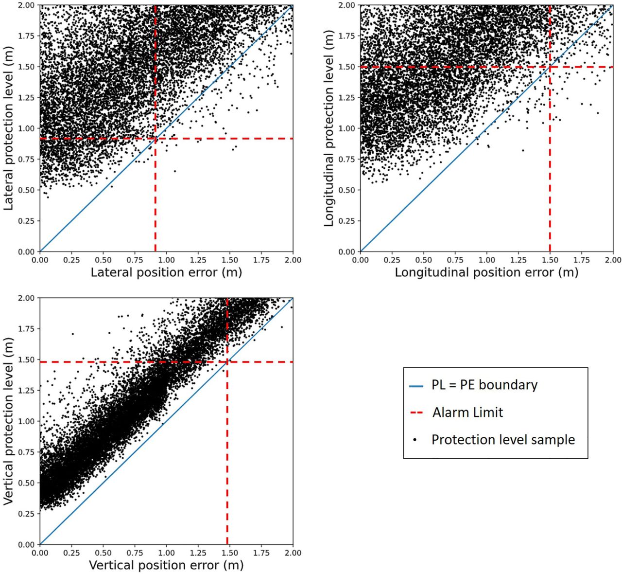
Figure 7 displays the integrity diagrams generated after the Stanford-ESA integrity diagram proposed for SBAS integrity (Tossaint et al., 2007). The diagram is generated from 15,000 samples of protection levels corresponding to randomly selected state estimates and camera images within the test sequence.

Integrity diagram results for the lateral, longitudinal, and vertical protection levels. The diagram contains protection levels evaluated across 15,000 different state estimates and camera images randomly selected from the test sequence. A majority of the samples are close to and greater than the position error magnitude, validating the applicability of the computed protection levels as a robust safety measure
For protection levels in each direction, we set the alarm limit (Table 1) based on the specifications suggested for mid-size vehicles in Reid et al. (2019), beyond which the state estimate is declared unsafe to use. The lateral, longitudinal, and vertical protection levels are greater than the position error magnitudes in ∼ 99% cases, which is consistent with the specified integrity requirement. Furthermore, a large fraction of the failures is in the region where the protection level is greater than the alarm limit and thus the system has been correctly identified to be under unsafe operation.
We conducted an ablation study to numerically evaluate the impact of our proposed epistemic uncertainty measure and outlier weighting method in computing protection levels. We evaluated protection levels in three different cases: Incorporating DNN covariance, epistemic uncertainty, and outlier weighting (VAR+EO); incorporating just the DNN covariance and epistemic uncertainty with equal weights assigned to all position error samples (VAR+E); and only using the DNN covariance (VAR).
For VAR, we constructed a Gaussian distribution using the DNN position error output and diagonal variance entries in each dimension. Then, we computed protection levels from the inverse cumulative distribution function of the Gaussian distribution corresponding to the specified value of integrity risk IR. Table 2 summarizes our results.
Evaluation of lateral, longitudinal, and vertical protection levels from our approach. We compare protection levels computed by our trained model using DNN covariance, epistemic uncertainty, and outlier weighting (VAR+EO); DNN covariance and epistemic uncertainty (VAR+E); and only using the DNN covariance (VAR). Incorporating epistemic uncertainty results in lower failure rate while incorporating outlier weights reduces bound gap and false alarm rate
Incorporating the epistemic uncertainty in computing protection levels improved the failure rate from 0.05 in lateral protection levels, 0.05 in longitudinal protection levels, and 0.03 in vertical protection levels to within 0.01 in all cases. This is because the covariance estimate from the DNN provides an overconfident measure of uncertainty, which is corrected by our epistemic uncertainty measure. Furthermore, incorporating outlier weighting reduced the average nominal bound gap by about 0.02 m in lateral protection levels, 0.05 m in longitudinal protection levels, and 0.05 m in vertical protection levels as well as false alarm rate by about 0.02 for each direction while keeping the failure rate within the specified integrity risk requirement.
The mean bound gap between the lateral protection levels computed from our approach and the position error magnitudes in the nominal cases is smaller than a quarter of the width of a standard US lane. In the longitudinal direction, the bound gap is somewhat larger since fewer visual features are present along the road for determining the position error using the DNN. The corresponding value in the vertical dimension is smaller, owing to the DNN’s superior performance in determining position errors and uncertainty in the vertical dimension. This demonstrates the applicability of our approach to urban roads.
For an integrity risk requirement of 0.01, the protection levels computed by our method demonstrate a failure rate equal to or within 0.01 as well. However, further lowering the integrity risk requirement during our experiments either did not similarly improve the failure rate or caused a significant increase in the bound gaps and the false alarm rate.
A possible reason is that the uncertainty approximated by our approach through both the aleatoric and epistemic measures fails to act as an accurate uncertainty representation for smaller integrity risk requirements than 0.01. Future research would consider more and varied training data, better strategies for selecting candidate states, and different DNN architectures to meet smaller integrity risk requirements.
A shortcoming of our approach is the large false alarm rate exhibited by the computed protection levels shown in Table 2. The large value results both from the inherent noise in the DNN-based estimation of position and rotation error as well as from frequently selecting candidate states that result in large outlier error values. A future work direction for reducing the false alarm rate is to explore strategies for selecting candidate states and mitigating outliers.
A key advantage offered by our approach is its application to scenarios where a direct analysis of the error sources in the state estimation algorithm is difficult, such as when feature rich visual information is processed by a machine learning algorithm for estimating the state. In such scenarios, our approach computes protection levels separately from the state estimation algorithm by both evaluating a data-driven model of the position error uncertainty and characterizing the epistemic uncertainty in the model outputs.
7 CONCLUSION
In this work, we presented a data-driven approach for computing lateral, longitudinal, and vertical protection levels associated with a given state estimate from camera images and a 3D LiDAR map of the environment. Our approach estimates both aleatoric and epistemic measures of uncertainty for computing protection levels, thereby providing robust measures of localization safety.
We demonstrated the efficacy of our method on real-world data in terms of bound gap, failure rate, and false alarm rate. Results show that the lateral, longitudinal, and vertical protection levels computed from our method enclose the position error magnitudes with 0.01 probability of failure and less than 1 m bound gap in all directions, which demonstrates that our approach is applicable to GNSS-denied urban environments.
HOW TO CITE THIS ARTICLE
Gupta S, Gao G. Data-driven protection levels for camera and 3D map-based safe urban localization. NAVIGATION. 2021;68:643–660. https://doi.org/10.1002/navi.445
ACKNOWLEDGMENTS
This material is based upon work supported by the National Science Foundation under award #2006162.
Footnotes
Funding information
NSF, Grant/Award Number: #2006162
- Received October 19, 2020.
- Revision received April 13, 2021.
- Accepted July 15, 2021.
- © 2021 Institute of Navigation
This is an open access article under the terms of the Creative Commons Attribution License, which permits use, distribution and reproduction in any medium, provided the original work is properly cited.


Jump to section
Related Articles
Cited By...
- No citing articles found.