

Abstract
Observation of terrestrial GNSS interference (jamming and spoofing) from low Earth orbit (LEO) is a uniquely effective technique for characterizing the scope, strength, and structure of interference and for estimating transmitter locations. Such details are useful for situational awareness, interference deterrence, and the development of interference-hardened GNSS receivers. This paper presents the results of a three-year study of global interference, with emphasis on a particularly powerful interference source active in Syria since 2017. It then explores the implications of such interference for GNSS receiver operation and design.
1 INTRODUCTION
This paper presents the results of a three-year study of terrestrial GNSS interference as observed through a software-defined GNSS receiver operating since February 2017 on the International Space Station (ISS). The fast, orbital, TEC, observables, and navigation (FOTON) receiver, developed by The University of Texas at Austin (UT) and Cornell University, is part of a larger science experiment called GPS Radio Occultation and Ultraviolet Photometry—Colocated (GROUP-C), an unclassified experiment aboard the ISS that is part of the Space Test Program—Houston Payload 5 (STP-H5) payload. Serendipitous observations of GNSS interference in the occultation data are an important early result of GROUP-C’s scientific objective to characterize GPS signals in the LEO environment. This paper discusses the interference signals detected, their effects, and interference mitigation strategies for receivers deployed in LEO and terrestrial environments.
The FOTON receiver is a science-grade spaceborne dual-frequency (GPS L1 and L2) GNSS receiver (Lightsey et al., 2014). Three levels of FOTON data are available for interference analysis: (1) raw 5.7-Msps intermediate frequency (IF) samples output by the FOTON front-end’s analog-to-digital converter; (2) 100-Hz data-modulation-wiped complex correlation products; and (3) 1-Hz standard GNSS observables (pseudorange, carrier phase, and carrier-to-noise ratio 𝐶∕𝑁0).
Although spaceborne GNSS sensors have been used for remote sensing via radio occultation (Ao et al., 2009) and reflectometry (Jin & Komjathy, 2010), there is little public literature exploring their use for monitoring terrestrial GNSS interference. Isoz et al. (2014) characterized interference observed at a LEO satellite, and approximated the location for one source, but was mainly concerned with determining whether the interference had a detrimental impact on GPS-RO (radio occultation) meteorological products. The more recent survey of GNSS interference localization techniques in Dempster and Cetin (2016) makes no mention of single-receiver Doppler-based localization, whether space-based or not.
General time difference of arrival (TDOA) and frequency difference of arrival (FDOA) interference localization has been extensively studied (Amar & Weiss, 2008; Bhatti, 2015; Griffin & Duck, 2002; Ho & Chan, 1997; Pattison & Chou, 2000), and such techniques have been applied for terrestrial interference localization from geostationary orbit (Haworth et al., 1997; Ho & Chan, 1993; Smith & Steffes, 1989). Application of TDOA or FDOA for localization from LEO can be viewed as an extension of such demonstrations, with the lower-altitude orbits enabling the localization of much weaker signals. Interference localization using a single satellite has been explored in Kalantari et al. (2016), but only simulation results are presented, and these unrealistically assume perfect-tone interference with a known and constant frequency.
This paper makes three primary contributions. First, it improves on the global survey technique in Isoz et al. (2014) by compensating for predictable 𝐶∕𝑁0 variations in the detection test. Second, it presents the results of a three-year study of global GNSS interference, with emphasis on a powerful interference source active in Syria since 2017. Via Doppler positioning using the FOTON instrument on the ISS, an estimate of the transmitter’s location is obtained whose horizontal errors are less than 1 km with 99% confidence based on reasonable clock and noise models. Such an accurate localization of a GNSS interference source from LEO is without precedent in the open literature. Third, this paper explores the implications of interference of the type generated by the source active in Syria for GNSS receiver operation and design.
A preliminary version of this paper was published in Murrian et al. (2019). The current version focuses on the observed interference, extends the analysis period through June 2020, offers a more detailed analysis of localization accuracy, and includes a new section exploring implications for GNSS receivers.
2 SINGLE-SATELLITE TERRESTRIAL SOURCE GEOLOCATION
As a prelude to the presentation of results from the observation campaign, this section introduces and analyzes the Doppler-based technique employed to estimate the location of the interference source operating in Syria.
Assuming a carrier can be extracted from an interference signal, single-satellite-based transmitter geolocation is possible from Doppler measurements alone (Becker, 1992; Ellis et al., 2020). The analysis presented here emphasizes the effect of transmitter clock stability on geolocation accuracy.
Consider a static transmitter emitting a signal at the GPS L1 frequency as observed by a moving receiver. Let 𝜆 be the signal wavelength in meters,  as the unit vector pointing from the transmitter to receiver, expressed in Earth-centered, Earth-fixed (ECEF) coordinates, 𝒗R as the receiver velocity with respect to the ECEF frame and expressed in ECEF in m/s, and
  as the receiver clock frequency error in s/s, all at the time of signal receipt. Further, let
  be the transmitter clock frequency error in s/s at the time of signal transmission, and 𝑤 be a zero-mean Gaussian error term that models thermal noise, ionospheric and tropospheric delay rates, and other minor effects, in Hz. Then the observed Doppler frequency in Hz at the receiver can be modeled as:
 1
1
where 𝑐 is the speed of light in m/s. It is assumed that 𝒗R,  , and the receiver position are known (e.g., via a GNSS receiver co-located with the transmitted signal receiver). The unknowns in Equation (1) largely stem from transmitter position, which is embedded in
  and
and  . The former is modeled as an unknown constant and the latter as a random walk process that evolves as:
 2
2
Here, 𝑣(𝑡𝑘) is a discrete-time Gaussian random process with 𝔼[𝑣(𝑡𝑘)] = 0 and 𝔼[𝑣(𝑡𝑘)𝑣(𝑡𝑗)] = 2𝜋2ℎ‒2𝛿𝑡𝛿𝑘,𝑗, ∀𝑘,𝑗, where ℎ‒2 is the first parameter of the standard clock model based on the fractional frequency error power spectrum, as given in Brown and Hwang (2012); 𝛿𝑡 = 𝑡𝑘+1 ‒ 𝑡𝑘 is the uniform sampling interval; and 𝛿𝑘,𝑗 is the Kronecker delta.
A transmitter could introduce any level of complexity to carrier-phase frequency behavior (e.g., frequency modulation, frequency hopping). Such behaviors, if not discovered and appropriately modeled, would confound single-pass geolocation efforts. Here, it is assumed that a nominally-constant carrier frequency is intended by the transmitter and that it is operating in steady-state conditions. In fact, it will be assumed that ℎ‒2 is sufficiently small enough that  can be modeled as constant over a short (e.g., 60-second) data capture interval.
Based on the above Doppler measurement model, a batch maximum likelihood estimator (Crassidis & Junkins, 2011) can be developed to estimate the unknown transmitter position and a constant value for  from a collection of single-pass Doppler measurements. If Doppler measurements from multiple satellite passes are available, they can be combined for single-batch estimation provided that a new value of
  is estimated for each pass. In other words,
  is viewed as constant over each short capture interval but variable from capture to capture.
When  is modeled as constant over a capture interval, actual transmitter clock instability gives rise to Doppler measurement errors. The impact of such errors on geolocation accuracy has been analyzed via the Monte Carlo simulation for three levels of transmitter clock quality, from a temperature-compensated crystal oscillator (TCXO) to a laboratory-grade oven-controlled crystal oscillator (OCXO). Simulation parameters were based on the real-world interference capture discussed in the next section: the true transmitter location was simulated to be 35.4 N latitude, 35.95 E longitude, 48 m altitude; the receiver trajectory was taken from the ISS orbit during the first 60 seconds of the capture interval on day 144 of 2018 (resulting in 441.65 km of total receiver displacement); and the measurement rate was 20 Hz.
First, an error-free Doppler time history was generated based on this scenario. Then, for each instance of the Monte Carlo simulation, an independent realization of a Doppler error random process consistent with the clock model being analyzed was generated and added to the error-free Doppler. Doppler error was modeled as a random walk process consistent with Equation (2). These models assume a smooth compensation for temperature control, such as is common for TCXOs used in GNSS receivers. Additionally, ℎ‒2 is assumed to dominate frequency stability over each short capture interval.
1,000 Monte Carlo trials were conducted for each of the three clock quality levels. Transmitter horizontal location estimation errors were observed to be zero-mean and apparently Gaussian, and they were consistent with the formal error ellipses of the associated linear least-squares estimator. To determine whether 1,000 trials were sufficient for a confident error analysis, subgroups of 250 trials were randomly selected from the 1,000 trials and each of their geolocation error ellipses were calculated.
Those subgroup samples were observed to deviate less than ±10 from the population mean with 99% empirical confidence. For example, 99% of the subgroups for the TCXO simulation had geolocation error ellipse estimates between 6, 900 ± 660 meters for the semi-major axis, and 690±71 meters for the semi-minor axis. Out of the 1×10⁵ subgroup samples drawn for each clock quality level, none were observed that deviated more than 17% from the population mean. Thus, 1,000-trial-based error ellipses for each clock quality level given in Table 1 can be assumed to be no more than 15% smaller, on either axis, than the error ellipses that would be produced in the limit of an infinite number of trials.
Marginal contribution of transmitter frequency instability to a single-pass geolocation error ellipse; the size of the 95% horizontal geolocation error ellipse, in meters, is characterized by the (a) semi-major and (b) semi-minor axes
Table 1 shows that the marginal contribution of transmitter frequency instability to single-pass geolocation error grows precipitously with reduced transmitter clock quality. These results suggest that single-pass geolocation of a TCXO-based transmitter is marginal at best, and could be even worse if the ℎ‒2 values for TCXOs in Table 1 are optimistic. On the other hand, if the transmitter is driven by an OCXO-quality clock, then clock instability contributes less than 720 meters (low-quality OCXO) or 67 meters (standard-quality OCXO).
The error ellipse characterized by 𝑎 and 𝑏 in Table 1 is highly eccentric, with the semi-minor axis oriented in the direction of satellite motion (e.g., if the satellite is moving west to east then transmitter location would be best resolved in that direction). It follows that additional satellite passes provide the most benefit when, relative to the transmitter location, they are geometrically dissimilar to previous passes.
3 ANALYSIS OF INTERFERENCE FROM SYRIA
This section presents an in-depth analysis of a particular interference source active on the east coast of the Mediterranean Sea during the period of this paper’s study, which spans from March 2017 to June 2020. The analysis illustrates techniques that can be applied generally to study terrestrial GNSS interference sources using signals collected in LEO.
Recording raw intermediate frequency (IF) data in LEO and relaying these to the ground for processing is an especially flexible approach well suited to studying new or poorly-understood interference. For the case presented here, the FOTON receiver captured 1-minute intervals of raw 5.7-Msps two-bit-quantized IF samples at GPS L1 (1,575.42 MHz) and GPS L2 (1,227.6 MHz) frequencies. These data were packaged and downlinked via NASA’s communications backbone. Ground processing using the latest version of UT’s software-defined GNSS receiver (Humphreys et al., 2020) enabled analysis and tracking of all radio frequency signals near GPS L1 and L2.
The following observations are based on signals captured on three days in the first half of 2018 along the ground tracks shown in Figure 1.

Ground tracks for interference-affected captures on days 74, 144, and 151 of 2018; each capture spans approximately 60 seconds; and the estimated transmitter location is marked on the west coast of Syria
3.1 Overview
Strong interference is present in both the L1 and L2 bands, but the nature of the interference is markedly different between the two bands. At L2, the interference is narrowband, whereas at L1, it is a wideband spread-spectrum signal. The L1 interference is a composite of individual signals with a common carrier centered near GPS L1 but each having a unique GPS L1 C/A pseudorandom number (PRN) spreading code. Such interference can be categorized as matched-code GNSS interference (Humphreys, 2017; Psiaki & Humphreys, 2020). Signals corresponding to almost all GPS L1 C/A PRN codes from 1 to 32 have been detected. When tracked by the UT software-defined GNSS receiver, all false signals exhibit 𝐶∕𝑁0 values greater than 40 dB-Hz. No discernible navigation data are modulated on the false GPS L1 signals. Moreover, the false signals are not clean simulated GPS L1 C/A signals; they exhibit unexplained fading and spectral characteristics. No false Galileo BOC(1,1) signals were detected in the L1 band.
The lack of navigation bit modulation renders the signals ineffective at spoofing, but matched-code interference is a particularly potent form of jamming (Humphreys, 2017). Why different techniques were used at L1 and L2 is unknown.
While some authentic GPS L1 C/A signals in the data are effectively jammed, the majority of authentic signals are still trackable owing to sufficient separation of corresponding false and authentic signals in code-Doppler space. Thus, a correct receiver navigation solution can still be formed despite the interference.
3.2 Power spectral characteristics
Figures 2 and 3 illustrate the captured signals’ spectral characteristics. The spectra of narrowband interference near L2 are simple and remain similar across all three days, but the wideband interference at L1 is more complex and variable. It is clear from the left column of Figure 2 that the matched-code interference is cluttered by other components. Were it generated by a high-quality signal simulator, L1 interference would tend to be smooth like the authentic signals underlying the spectrum shown in the lower left panel of Figure 2. Instead, it appears to be an amalgam of components. Figure 3 reveals that the rounded prominence in the L1 Day 144 panel exhibits oscillatory behavior with a 5-second period. Whether such variations are deliberate or caused by transmitter idiosyncrasies is unknown.
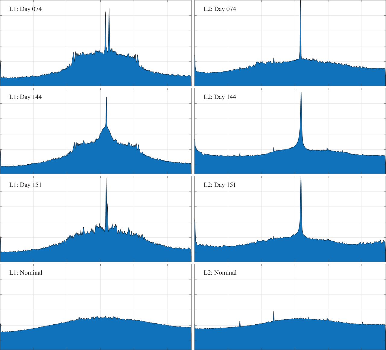
Power spectra centered near the GPS L1 (left column) and L2 (right column) frequencies from interference-affected data captured on days 74, 144, and 151 of 2018 (top three rows), and from nominal data captured on day 158 of 2018 (bottom row); the frequency span is approximately 3 MHz wide, scaled linearly with 0.5 MHz divisions; all ordinate axes are in dB and scaled equivalently for ease of comparison; and spectra are estimated by Welch’s method (Welch, 1967) from 1-second data intervals with a 5.6-kHz frequency resolution

Power spectra near L1 for the day 144 capture showing maximum (top) and minimum (bottom) phases of the waxing and waning wideband (∼ 0.25MHz) central interference prominence; the prominence oscillates with a period of approximately 5 seconds. The L1: Day 144 plot in Figure 2 catches the prominence waning 2 seconds after the maximum shown in the top plot
3.3 Baseband signal characteristics
Figure 4 shows time histories of 10-ms accumulated complex correlation products from a false (top panel) GPS L1 C/A signal and two authentic (bottom two panels) GPS L1 C/A signals present in the captured L1 band. The false signal’s empirical 𝐶∕𝑁0 value is 42.5 dB-Hz on average, but the signal is highly irregular, manifesting both gradual and sudden fading. The gradual fading may be a result of scintillation as the signal passes upward through the lower ionosphere (Humphreys et al., 2010), but the sudden fading, highlighted in the inset of the top panel, is unnatural and likely originates at the transmitter.

In-phase (black) and quadrature (gray) 10-ms accumulation time histories for the strongest false signal from the day 74 capture (top), the strongest authentic signal from the day 74 capture (middle), and the strongest signal from day 158 nominal capture (bottom); data wipe-off was implemented in the middle and bottom figures. The inset on the top panel shows an amplified view of two sudden amplitude fades in the received false signal. The maximum carrier-to-noise ratio 𝐶∕𝑁0 over the intervals shown are, from the top, 42.5, 46.8, and 52.5 dB-Hz, respectively

Top: Doppler time history corresponding to the false PRN 10 signal from the day 144 capture; Bottom: Post-fit residuals of the Doppler time history assuming the estimated transmitter location and clock rate offset (the standard deviation of the post-fit residuals is 2.3 Hz)
3.4 Source geolocation
The presence of a trackable carrier signal after despreading (compare to the top panel of Figure 4) enables geolocation of the interference source as described in Section 2. A receiver navigation solution was first estimated on days 74, 144, and 151 of 2018 using an extended Kalman filter (EKF) drawing in pseudorange and Doppler measurements extracted from the authentic GPS L1 C/A, GPS L2C, and Galileo E1 signals. Propagation of the receiver state estimate between measurement updates was based on a nearly-constant acceleration dynamics model. Time histories of the quantities 𝒗R,  , and the receiver position component of
  were then extracted from the EKF’s state estimate and treated as known for purposes of source geolocation.
A batch estimator for interference source position and clock frequency bias was formulated as described in Section 2. It was assumed that the interference observed on all three days originated from the same stationary transmitter, which allowed multiple days of Doppler measurements, collected on non-repeating ground-tracks, to be combined to form a tightly-constrained estimate. If these assumptions were false, large post-fit measurement residuals could be expected to manifest, although this was not the case. Consistent with the assumption of a stationary transmitter, transmitter altitude was assumed to be near ground-level and was included as a pseudo measurement.
A constant transmitter clock frequency error  was assumed to apply during each capture, but a new value of
  was estimated for each of the three captures. Comparing the batch-estimator-produced estimates of
  for days 74 and 144 revealed a two-sample transmitter clock frequency stability of approximately 𝜎𝑦(2,𝑇,𝜏) = 6.85 × 10‒9 at a sampling interval 𝑇 of 70 days and an observation time (averaging interval) 𝜏 of approximately 50 seconds. The 𝐵2 bias function (Barnes, 1969) was used to convert this two-sample deviation to an Allan deviation, where 𝐵2(𝑟, 𝜇) = 1.8144 × 10⁵ for 𝑟 = 𝑇∕𝜏 and 𝜇 = 1, which assumes ℎ‒2 is the dominant spectral component. This yielded an equivalent Allan deviation for 𝜏 = 50 seconds of 𝜎𝑦(2,𝜏,𝜏) = 1.6×10‒11, which is consistent with a standard-quality OCXO (Bagala et al., 2016).
Thus, given the results of Table 1, treating  as constant over each 60-second capture can be conservatively expected to introduce 95% errors smaller than 720 meters (that corresponding to a low-quality OCXO) in single-pass geolocation. A Monte-Carlo simulation like the one that produced the Table 1 data but for the combined three days of collection showed that, assuming independence in the clock frequency errors between passes, and conservatively assuming a low-quality OCXO, this error source can be expected to contribute 95% errors below 230 meters in the combined 3-day solution.
It is worth noting that, because  and
and  enter equivalently into the Doppler measurement model (1), and because no prior knowledge of these parameters is assumed in the batch maximum-likelihood estimator, an error in the EKF’s estimate of
  will directly manifest in the batch-estimator-produced estimate of
  for each capture. However, examination of the the EKF’s error covariance revealed that its estimate of
  was good to better than 7×10‒10 (1-𝜎) for the day 74 and 144 captures. Thus, receiver-side errors are likely small enough that 𝜎𝑦(2,𝜏,𝜏) = 1.6 × 10‒11 remains an accurate assessment of the transmitter clock stability.
Figure 5 shows time histories of Doppler and post-fit residuals for false PRN 10 collected on day 144. The standard deviation of the post-fit residuals is 2.3 Hz, indicating that the measurement model in Equation (1) and the assumption of a constant  over each capture are reasonably accurate. Figure 6 shows the estimated position of the interference source. The horizontal error ellipses, which indicate a solution better than 220 meters (95%), are formal error ellipses assuming (1) constant
  over each capture, (2) a standard deviation of 5 m for the transmitter altitude constraint, and (3) a standard deviation between 2.3 and 2.5 Hz (depending on the empirical post-fit residuals for each capture) for the measurement error 𝑤 from (1). Assuming an OCXO-quality clock in the transmitter, the error caused by modeling a constant
  is small compared to these formal error ellipses. While the true location is not known, the geolocation solution based on the model plausibly coincides with a Russian-operated air base in Syria.

Estimated transmitter location overlaid on formal-error 95% and 99% horizontal error ellipses; the location is coincident with an airbase on the coast of Syria. The semi-major axis of the 95% ellipse is 220 meters
3.5 Transmitter power
In the presence of interference, 𝐶∕𝑁0 actually measures the carrier-to-interference-and-noise ratio (CINR). By analyzing the authentic signal CINR values in the captured data, one can infer the transmitted power in the direction toward the ISS of the emitter located in Syria. The data presented here are for the day 74 capture. The average decrease in the CINR values observed at the ISS when 1,340 km from the source was approximately 6 dB.
One may assume the interference acts as multi-access interference, whose spectral density is 𝐼0 = (2∕3)𝑃I𝑇𝐶 (Humphreys, 2017), where 𝑃I is the received interference power and 𝑇𝐶 = 1023‒1 ms is the GPS L1 C/A spreading code chip interval. Then, assuming 𝑁0 = ‒204 dBW/Hz, a drop in CINR by 6 dB implies 𝑃I = ‒137 dBW. Let 𝑃S = 𝑃I ‒𝐺𝑟 +𝐿, and assume path loss 𝐿 = 159 dB, consistent with a stand-off distance of 1,340 km, and receiver antenna gain 𝐺𝑟 = 3 dB.
It follows that the transmitter power of the interference source in the direction toward the ISS during the day 74 capture is 𝑃S = 19 dBW, or 79 W. If the transmitter is focused on ground-based targets, then it is possible that the gain pattern is toroidal. The elevation angle of the ISS as seen from the transmitter is low during this period (varying between 8 and 13.5 degrees) and may have been near the maximum of a toroidal gain pattern.
4 GLOBAL INTERFERENCE SURVEY VIA RECEIVER-REPORTED CINR
The raw IF data captures from the ISS FOTON receiver enabled detailed monitoring of GNSS interference signals and their structure, but such captures are infrequent and limited to short 1-minute intervals. By contrast, the 1-Hz standard GNSS observables and 100-Hz data-wiped complex correlation products have been logged nearly continuously since early 2017. These data facilitate a worldwide survey of strong GNSS interference.
4.1 Calculation of receiver-reported CINR
Receiver-reported CINR is calculated as:
 3
3
where the expectation 𝔼[𝐼2 +𝑄2] is estimated by moving average using a Euler approximation to a standard low-pass filter:
 4
4
with subscripts 𝑘 and 𝑘 ‒ 1 indicating the current and previous accumulation interval. The gain parameter  with accumulation interval 𝑇𝑎 = 10 msec and filter time constant 𝜏 = 0.5. 𝐼𝑘 and 𝑄𝑘 are the in-phase and quadrature prompt correlation products for the current accumulation interval.
The receiver noise floor,  , can be derived analytically for a 2-bit quantizing RF front-end and a software-defined GNSS receiver based on the quantization models of both the RF front-end and receiver local carrier replica. It can be shown that:
 5
5
where 𝑁 is the number of samples per accumulation interval, 𝑎0, 𝑎1, 𝑏0, and 𝑏1 are the low and high quantization values of the RF front-end and local carrier replica, respectively, and 𝑝𝑎0, 𝑝𝑎1, 𝑝𝑏0, and 𝑝𝑏1 are their associated probabilities, respectively.
In practice, 𝑝𝑎0 and 𝑝𝑎1 depend on the implementation of the automatic gain control (AGC) in the RF front-end, and 𝑝𝑏0 and 𝑝𝑏1 are selected by the receiver designer (e.g., to minimize quantization distortion). The following values are applicable to the FOTON receiver:

which yield a noise floor of  front-end units.
4.2 Methodology
The carrier power 𝐶 of an authentic signal can be modeled as a function 𝐶(𝑗, 𝑓, 𝑟𝑠𝑟,𝑧𝑠,𝑧𝑟), where: 𝑗 is the GNSS satellite identifier (SV ID); 𝑓 is the frequency band (L1 or L2); 𝑟𝑠𝑟 is the range between the GNSS satellite antenna and the ISS FOTON antenna; 𝑧𝑠 is the angle between the satellite boresight direction and the direction to the ISS antenna (i.e., the satellite antenna off-boresight angle); and 𝑧𝑟 is the angle between the ISS antenna boresight direction and the direction to the satellite (receiver antenna off-boresight angle).
A hypothesis test based on the receiver-reported CINR can be designed to detect whether (𝐻1) or not (𝐻0) the receiver is experiencing interference. Under a given 𝑃F, this requires that the statistics 𝔼[𝑙|𝐻0] and Var(𝑙|𝐻0) be known. To obtain these statistics, this section assumes the receiver reports interference-free data (consistent with 𝐻0) when the ISS is over deep ocean bodies.
To isolate the variations in reported CINR due to interference, the data are first pre-processed to eliminate the predictable sources of carrier power variation. First, the dependence of 𝐶 on 𝑟𝑠𝑟 is removed by compensating for the free space path loss:

Modeling of interference-free 𝐶∕𝑁0 is complicated by the ISS’s local multipath environment. The ISS antenna is flanked by solar panels that move with respect to the FOTON antenna, causing a non-stationary signal obstruction and multipath environment. Nevertheless, an off-boresight angle window 𝑧𝑟 ∈ [0◦,15◦] is known to be free of obstructions. Only the signals received in this window are considered for interference detection in this paper’s analysis. Confining 𝑧𝑟 to this window restricts the geometry between GNSS satellites and the ISS such that 𝑧𝑠 ∈ [14.2◦, 15.2◦] (see Figure 7). The GNSS antenna gain pattern can be assumed to be relatively constant over ±0.5◦. Thus, Ĉ(𝑗, 𝑓, 𝑧𝑠,𝑧𝑟) can be assumed independent of 𝑧𝑠.

For receiver off-boresight angle 𝑧𝑟 ≤ 15◦ (within the gray region), the satellite off-boresight angle 𝑧𝑠 is restricted between 14.2◦ ≤ 𝑧𝑠 ≤ 15.2◦
The mean and variance of ISS-reported range-compensated-CINR values Ĉ∕𝑁0 collected over deep ocean regions are maintained as control data in a three-dimensional grid of SV ID 𝑗, frequency band 𝑓, and receiver off-boresight angle 𝑧𝑟. For a worldwide analysis of GNSS interference events, a hypothesis test is performed on the test statistic derived from Ĉ∕𝑁0 values that fall within 𝑧𝑟 ∈ [0◦,15◦]. The test is performed separately for the L1 and L2 bands since the interference characteristics are frequency-dependent. If the reported test statistics fall below  , the receiver is declared to be under interference. This threshold respects a 𝑃F of approximately 1.35 × 10‒3.
4.3 Discussion of results
Figure 8 shows the ratio of the number of potential interference events recorded at L1 (top panel) and L2 (bottom panel) to the total number of hypothesis tests performed at each location for the foregoing detection threshold. As expected, a high ratio of potential interference events is reported for both L1 and L2 near Syria (marked with a red dot). Note that the interference hotspot appears to the east of the source because the ISS orbit is prograde and the FOTON antenna points in the anti-velocity direction. In other words, the FOTON antenna is exposed to interference only after the ISS passes eastward over an emitter’s location.

Ratio of number of potential GPS L1 (top panel) and L2 (bottom panel) interference events recorded to the total number of hypothesis tests performed at each location on the map for the full span of data considered in this paper, from March 2017 to June 2020. The red dots indicate the estimated origin of the interference from Syria based on raw IF recordings. Another hotspot of interference is apparent to the west of the Syrian location. The magenta dots denote the approximate location of GNSS interference reports in the Libyan region (United States Coast Guard). In addition to the interference over the Syrian and Libyan regions, strong L2 interference over mainland China is observed. The green dot at (32◦ N, 114◦ E) indicates a hypothesized interference source location based on the shape and location of the observed hotspot
The high values of the statistic for both L1 and L2 east of Syria indicate that the interference activity in Syria has been persistent over nearly the full interval considered in this paper, from March 2017 to June 2020. A monthly analysis (not shown) revealed that the source has been transmitting at L2 since no later than March 2017. It began transmitting weak interference at L1 during the second half of 2017, then much stronger interference at L1 during the first quarter of 2018. The interference at L1 and L2 was ongoing as of June 2020.
An additional hotspot is present to the west of the Syrian location. This hotspot, which emerged in the second half of 2019, is consistent with reports of GNSS interference in the Libyan region (United States Coast Guard, n.d.). The magenta dots in Figure 8 denote the approximate location of the area in which interference has been documented (33◦ N, 14◦ E). Figure 8 also reveals strong L2 interference over mainland China. This interference has been present since March 2017 at the latest and was ongoing in June 2020. The green dot in Figure 8, marked at (32◦ N, 114◦ E), indicates a hypothesized interference source location based on the shape and location of the observed hotspot.
Note that the method of counting potential interference events based on CINR degradation ignores cases where interference might lead to complete loss of track of some or all GPS signals. However, the data from the ISS shows that FOTON does not lose track of authentic GNSS signals even when flying by the strong interference source in Syria. In fact, the reported CINR over Syria is well above the weakest signal that FOTON is capable of tracking. As a result, it was concluded that in cases where FOTON seems to track few or no GPS signals, it is likely due to some abnormal behavior of the receiver, and not due to a potential interference event.
In addition to the global average analysis summarized in Figure 8, it is instructive to examine the time history of receiver-reported CINR as the ISS passes over an interference hotspot. Figure 9 shows two such histories for signals within the admissible range of 𝑧𝑟 as the ISS goes over the strong interference regions in Syria [Figure 9(a)] and China [Figure 9(b)]. Green and blue data points represent range-compensated CINR values for authentic L1 and L2 GNSS signals, respectively, above the applicable thresh-old, which depends on 𝑖, 𝑓, and 𝑧𝑟. Light red data points are the same data when below the applicable threshold. Both L1 and L2 signals are declared under interference in Figure 9(a), whereas only L2 signals are declared under interference in Figure 9(b). The brief dip in Figure 9(b) prior to the major dip over China is caused by the interference originating in Syria. Gaps in the time histories indicate periods with no tracked signals in the admissible off-boresight angle window.

Time histories of range-compensated receiver-reported CINR as the ISS flies over potential GPS interference zones over Syria and China
5 IMPLICATIONS FOR GNSS RECEIVERS
The matched-code interference captured over Syria is intriguing. So far as this paper’s authors are aware, no other GNSS interference captured from an operational (as opposed to experimental) source has exhibited the characteristics observed in the interference emanating from Syria. If the intent behind the signals transmitted at L1 is not spoofing, but rather denial of GPS service, as might be inferred from the lack of navigation data bit modulation, then it is unclear why an ensemble of signals, each one modulated by a separate GPS L1 C/A spreading code, was transmitted. The transmitter could just as well allocate its power to a single GPS L1 C/A spreading code, or any code with a similar spectral density. However, transmitting a multitude of spreading codes can be effective at disrupting cold-start acquisition of GPS L1 C/A signals, as explained below.
5.1 Efficient jamming
The art of jamming is more sophisticated than merely emitting RF energy into a target band. An efficient jammer is one that effectively disrupts GNSS service in a given area of operations but does so with as little power as possible. Such frugality extends the life of battery-powered jammers, and makes jammers less conspicuous.
The key to efficient jamming is avoiding wasteful allocation of signal power. Obviously, allocating power outside a target receiver’s passband is wasteful because the interference is filtered out by the receiver’s RF front-end. Less obviously, narrowband jamming applied directly in the passband is also wasteful.
To understand this, consider the vector space of all possible input signals, and a partitioning into a subspace that contains the jamming signal and one that does not. If the jammer-occupied subspace is sparse with respect to the desired signal subspace, and if the receiver’s front-end amplification and quantization are not saturated, then a technique can be developed to excise the jammer-occupied subspace with minimal degradation to the desired signals. For a narrowband jammer, the technique is notch filtering; for a pulsed jammer, the technique is pulse blanking (Humphreys, 2017).
An efficient jammer maximizes overlap with the desired-signal subspace for a given power allocation. Jamming that is continuous in the time domain and white (spectrally flat) within the desired signal passband in the frequency domain is reasonably efficient because it extensively overlaps the desired signal subspace. Continuous-time matched-spectrum jamming is even more efficient; instead of spreading the jamming power evenly across the passband, a matched-spectrum jammer shapes it for greater overlap with the desired signal subspace.
Consider a random binary spreading code with chip interval 𝑇C. Suppose a spectrally-flat jammer is designed to cover the spreading code’s primary spectral lobe and first two side lobes, for a total frequency span of 4∕𝑇C Hz. The noise power density that passes through the receiver’s matched filter is 𝐼0 = 𝑃I𝑇C∕4, where 𝑃I is the interference power. By contrast, for a matched-spectrum jammer 𝐼0 = (2∕3)𝑃I𝑇C (Humphreys, 2017). When 𝐼0 is large enough that CINR ≈ 𝐶∕𝐼0, the matched-spectrum jammer is 4.3 dB more potent than the spectrally-flat jammer. What is more, the spectrally-flat jammer spanning 4∕𝑇C Hz can be excised by filtering in the frequency domain: even if the main lobe and adjacent two side lobes of the authentic signals are removed along with the jamming, the authentic signals are only attenuated by 13 dB. The spectrally-flat jammer must spread its power even wider to avoid such excision by filtering, resulting in an even less favorable potency compared to matched-spectrum jamming. By contrast, a matched-spectrum jammer cannot be excised by filtering because its spectrum follows the sinc2(𝑓𝑇C) envelope of the authentic binary-code-modulated signals. Thus, spectrum matching is a necessary condition for efficient jamming.
However, spectrum matching is not a sufficient condition for effective jamming. Consider a jammer emitting a carrier modulated only by a single publicly-known spreading code of arbitrary length. This signal is sparse with respect to the desired signal subspace. It can be excised by the receiver generating a local replica of the interference signal, aligning this replica’s code phase, carrier phase, and amplitude with the interference signal, and subtracting the replica from the digitized output of the receiver’s RF front-end. Assuming sufficient front-end bit depth and amplifier linearity, this procedure can be extended to an arbitrary number of such interference signals, each with a known waveform; the technique is known as successive interference cancellation (SIC; Madhani et al., 2003).
Thus, an effective jammer will avoid predictable signals: a more sophisticated approach to spectrum matching is modulation of the carrier with a non-repeating spectrum-matching spreading code known only to the jammer. But this is only necessary when the target receiver is capable of SIC. If, for example, the receiver has no way of distinguishing authentic signals from interference signals, then it cannot apply SIC without also eliminating desired signals.
5.2 The cold start vulnerability
It is instructive to consider the conditions under which a GNSS receiver is unable to distinguish between authentic and interference signals: (1) the authentic and interference signals are identical in all aspects of significance (modulation, code phase, carrier phase and frequency, amplitude), or (2) the authentic and interference signals are identical except in ways the target receiver is unable to exploit to distinguish them. In case (1), the interference is hardly a problem: it simply reinforces the authentic signals. Case (2) is more interesting.
Let the term spoofing interference refer to matched-code interference with all additional modulation requisite to make the interference signal’s structure and content identical to an authentic signal’s. If a receiver is exposed to spoofing interference while already tracking enough authentic signals to form a navigation solution and when in possession of accurate satellite ephemerides, it can distinguish any authentic and interference signals that differ in code phase, carrier frequency, or amplitude. (It can additionally distinguish by carrier phase if performing precise carrier-based navigation.) Therefore, jamming a navigation-locked receiver with spoofing interference may be ineffective because the target receiver can apply SIC.
However, during a cold start, the target receiver’s time and position are uncertain, and it lacks the ephemerides necessary to predict the code phase and Doppler of authentic signals even if its time and position were known. In this case, the receiver is highly vulnerable to spoofing interference. Suppose a jammer generates a counterpart power-matched spoofing signal for each authentic GNSS signal available in an area of operations. Suppose further that the ensemble of spoofing signals is self-consistent with a location and time different from the target receiver’s true location and time.
On a cold start, the receiver is jammed, not in the traditional sense of being unable to acquire and track the authentic signals, but rather in the sense of being unable to confidently declare which of two plausible-looking navigation solutions is correct. If, under this circumstance, the receiver refuses to provide a navigation solution, the user is effectively denied GNSS service. If instead the receiver mistakenly provides the spoofed solution, the user could be exposed to hazardous, misleading information.
This type of spoofing interference is highly efficient. Suppose the target receiver has a cold-start CINR acquisition threshold of 𝜂 dB-Hz. Then traditional matched-spectrum jamming would require a jamming-to-authentic power ratio equal to:
 6
6
which, for GPS L1 C/A signals and a typical 𝜂 = 30 dB-Hz, amounts to 31.8 dB. By contrast, jamming via single-counterpart power-matched spoofing interference requires only 𝑃I∕𝐶 = 0 dB, which makes it more than 1,500 times more efficient for denial of GNSS service at cold start.
5.3 Discussion
The interference captured over Syria causes traditional matched-spectrum jamming at close range, and is capable of disrupting cold-start acquisition far beyond this (along its line-of-sight). Indeed, it would be at least partially effective at preventing FOTON cold start even at the maximum line-of-sight range to the ISS, or approximately 1,600 km. However, the interference signals as broadcast have at least four flaws, any one of which could be exploited by receivers to distinguish them from authentic signals: (1) they lack navigation data modulation; (2) they are broadcast on a common and constant carrier frequency; (3) they share a common code phase alignment; and (4) they include signals for (almost) all GPS PRNs. A receiver built to detect these anomalies could identify the imposter signals and eliminate them via SIC.
However, in general, spoofing interference is not so easily distinguished from authentic signals, and can be both effective and power-efficient at denying GNSS service on cold start. The best defense against spoofing interference intended to deny GNSS service remains an open problem.
6 CONCLUSIONS
Low-Earth-orbiting instruments capable of receiving signals in GNSS bands are a powerful tool for characterizing GNSS interference emanating from terrestrial sources. Data from one such instrument, the FOTON software-defined GNSS receiver, which has been operational on the International Space Station since February 2017, reveal interesting patterns of GNSS interference from March 2017 to June 2020. Signals from a particularly powerful and persistent interference source active in Syria since 2017 were captured and characterized, and the source was geolocated to better than 1 km. A global analysis revealed other interference hotspots around the globe in both the GPS L1 and L2 frequency bands. Matched-code interference such as emitted at the GPS L1 frequency by the jammer in Syria is power-efficient for jamming signal-locked GNSS receivers. GNSS receivers are particularly vulnerable to such interference during cold start.
HOW TO CITE THIS ARTICLE
Murrian MJ, Narula L, Iannucci PA, et al. First results from three years of GNSS interference monitoring from low Earth orbit. NAVIGATION. 2021;68:673–685. https://doi.org/10.1002/navi.449
ACKNOWLEDGMENTS
Work at The University of Texas has been supported in part by the National Science Foundation under Grant No. 1454474 (CAREER) and in part by the U.S. Department of Transportation (USDOT) under Grant 69A3552047138 for the CARMEN University Transportation Center (UTC). Work at the Naval Research Laboratory was supported by the Chief of Naval Research. The STP-H5/GROUP-C experiment was integrated and flown under the direction of the Department of Defense Space Test Program.
Footnotes
Funding information
U.S. Department of Defense Space Test Program; U.S. Naval Research Laboratory; National Science Foundation, Grant/Award Number: 1454474; U.S. Department of Transportation, Grant/Award Number: 69A3552047138
- Received September 2, 2020.
- Revision received May 7, 2021.
- Accepted September 2, 2021.
- © 2021 Institute of Navigation
This is an open access article under the terms of the Creative Commons Attribution License, which permits use, distribution and reproduction in any medium, provided the original work is properly cited.


Jump to section
Related Articles
Cited By...
- No citing articles found.