

Abstract
This paper presents a random forest-based machine learning algorithm to automatically detect satellite oscillator anomalies using dual- or triple-frequency GPS carrier phase measurements. The algorithm can distinguish satellite oscillator anomalies from other GPS carrier phase disturbances including ionospheric scintillation and receiver oscillator anomalies. Carrier phase power spectral density and carrier phase ratios between carriers are extracted from measurements and applied as input features to the random forest algorithm. The method is trained using data collected at seven GNSS monitoring stations located in Alaska, Ascension Island, Greenland, Hong Kong, Peru, Puerto Rico, and Singapore. The overall detection accuracies of 98.4% and 99.0% are achieved for dual- and triple-frequency signals, respectively. The method outperforms other machine learning algorithms. The preliminary detection results demonstrate that the method presented can be employed on a global satellite oscillator anomaly monitoring system.
- global monitoring system
- GPS
- machine learning
- phase scintillation
- random forest
- satellite oscillator anomaly
- signal quality monitoring
- support vector machine
1 INTRODUCTION
GNSS signal-in-space (SIS) quality is fundamental to the operation and accuracy of the position, navigation, and timing (PNT) solutions provided by GNSS. The stability of the onboard oscillators is of paramount importance as they provide the signal time-of-transmission for satellite-receiver range measurements.
Satellite oscillator anomalies are manifested as SIS carrier phase disturbances. Their occurrence may be led by changes in state of the satellite clock (Blanch et al., 2013; Walter et al., 2003; Walter et al., 2012). Large anomalies may lead to the degradation of precision, service discontinuity, loss of augmentation correction service such as the Wide Area Augmentation System (WAAS), or even outage, ultimately impacting the accuracy and integrity of GNSS applications (Gordon et al., 2009; Liu & Morton, 2019, 2020a, 2020b; Vary, 2012).
Therefore, it is important to monitor and provide a timely warning of anomaly occurrence. In addition, the characterization of the anomaly occurrence will help to improve monitoring systems’ performance (Heng, 2012) and enable investigation of the cause of these events, where there is a lack of understanding due to the availability of anomaly data (Cobb et al., 1995). Furthermore, the characterization also provides guidance on future navigation satellite systems and satellite oscillator design in order to avoid these glitches, which is of great interest to the GPS satellite manufacturer (e.g., GPS III [Lockheed Martin, n.d.]).
Satellite oscillator anomalies have been investigated in several past studies (e.g., Benton and Mitchell [2012, 2014], Liu and Morton [2020b]). Benton and Mitchell (2012) observed pulses of rapid phase variations at GPS L1 caused by a satellite oscillator anomaly. In Benton and Mitchell (2014), a modern GPS Block IIF satellite (PRN 1) showed sequences of oscillator anomalies (with a maximum phase deviation larger than one cycle) on October 26, 2012. In Liu and Morton (2020b), frequent micro satellite oscillator anomalies (with a maximum phase deviation around 0.2 cycles) were observed from multiple GPS Block IIF satellites.
To offer a timely warning of these anomalies for the users, in particular for safety-critical services with the most stringent requirements such as aircraft navigation (Vioarsson et al., 2001; Weiss et al., 2010), a global satellite oscillator anomaly monitoring system is desired, and the capability of automatic detection is an important requirement (Gordon et al., 2009; Shallberg & Sheng, 2008).
Heo and Cho (2012) proposed using the Teager Energy operator to detect oscillator anomalies by identifying sudden changes. They assumed that using dual-frequency measurements or the Klobuchar model could remove the ionospheric effect such that any sudden, detected changes were contributed by the oscillator anomaly. However, these assumptions are not valid when there is ionospheric scintillation.
Ionospheric scintillation is typically due to a refractive or diffractive effect as GNSS signals propagate through ionospheric irregularities. The diffractive effects introduce random carrier phase fluctuations, which cannot be removed by dual-frequency measurements or ionospheric models (Carrano et al., 2013; McCaffrey & Jayachandran, 2019; Morton et al., 2020). Therefore, this approach is not always effective. To accommodate the problem, two (or more) nearby receivers were also utilized to distinguish the satellite oscillator anomaly from ionospheric scintillation and receiver oscillator anomalies (Gordon et al., 2009; Hansen et al., 1998; Ramesh et al., 2017). A satellite oscillator anomaly is identified by observing the same anomaly from two (or more) receivers. Two major shortcomings of this approach are that the requirement of two or more receivers makes it difficult to apply to existing monitoring and any updates to existing systems would be costly.
Liu and Morton (2019, 2020a, 2020b) proposed a machine learning (ML)-based satellite oscillator anomaly detection method using a single receiver. It involves three stages: detection of the phase disturbance using a linear kernel support vector machine (SVM); differentiation of the oscillator anomaly from ionospheric scintillation using the frequency dependence property and a radial basis function (RBF) kernel SVM; and differentiation of the satellite oscillator anomaly from receiver oscillator anomaly by examining the detected phase disturbances on different satellites at the same receiver. The two independent classification methods used in the first two stages result in suboptimal performance as the two detection stages are not end-to-end optimized.
In this paper, we propose a random-forest-based ML approach to replace the first two stages of the method discussed by Liu and Morton (2019, 2020a, 2020b). The random forest architecture is implemented to solve a classification problem with three classes: oscillator anomalies, ionospheric scintillation, and no disturbances. Features used in the ML algorithm include carrier phase power spectral density (PSD) and ratios of the carrier phase measurements. Both dual- and triple-frequency GPS carrier phase measurements are used to demonstrate that this random-forest-based ML method outperforms the approach presented by Liu and Morton (2020b) for the task of oscillator anomaly detection in terms of accuracy and number of detected anomaly events. In this paper, the same approach used by Liu and Morton (2020b; the third step in the algorithm) is applied to the identified oscillator-induced phase disturbances to differentiate a satellite oscillator anomaly from a receiver oscillator anomaly.
The rest of the paper is organized as follows: Section 2 introduces the methodology of the satellite oscillator anomaly detection; Section 3 evaluates the performance of the detection method; preliminary detection results are presented in Section 4; and finally, concluding remarks and future work are presented in Section 5. Note that we use the terms scintillation and phase scintillation interchangeably in this paper, where both terms refer to carrier phase scintillation.
2 METHODOLOGY
The method presented in this paper consists of two stages. First, a random-forest-based ML algorithm is implemented to detect any oscillator anomalies by differentiating them from ionospheric scintillation and quiet time cases. Second, the differentiation between satellite oscillator anomalies and receiver oscillator anomalies is conducted using the same approach as discussed by Liu and Morton (2020b).
A block diagram is shown in Figure 1 to illustrate the process. In this section, we will provide a brief summary of the random-forest algorithm, followed by the ML architecture for oscillator anomaly detection. Finally, the distinction between satellite and receiver oscillator anomalies is summarized for the sake of completeness.

Satellite oscillator anomaly detection block diagram
2.1 Decision Tree and Random Forest
Random forest is a supervised ML algorithm suitable for classification tasks (Breiman, 2001; Fernandez-Delgado et al., 2014). It makes a decision by majority vote from a group of decision trees, in which each decision tree makes their prediction independently.
The building block of the random forest is the decision tree. Assume a dataset of size n: {(xi, yi)}, i = 1,…, n, where the tuple (xi, yi) represents the i-th sample. For each sample, x ∈ Rm represents the m-dimensional features and y is the corresponding label. The goal of a decision tree is to learn a mapping function g from the training dataset such that the predicted label ŷ = g(x) matches the actual label y as accurately as possible.
Figure 2 shows an example decision tree for a three-class classification task. The left subplot shows the feature domain of the data set. Each dot/triangle/cross represents a data sample, where each sample has two features (x1, x2). The blue dot, red cross, and black triangle represent label a, b, and c, respectively. The dashed lines denote the decision boundaries, which are determined in the training process. The trained decision tree is shown on the right subplot where each leaf node is marked with a label, which is also determined in the training process.

Illustration of a decision tree for a three-class classification task
The decision/classification of a data sample is made by traversing the tree from top to bottom. At each node, a subtree is selected based on comparing the feature value of the data sample to the threshold of that node. This process is repeated until the leaf node is reached. Then the predicted label is the corresponding label of the leaf node. The training process of the decision tree is to recursively find the best split for each node, where the feature and the corresponding threshold for that best split are recorded (Bishop, 2006; Quinlan, 1986).
A decision tree may achieve excellent classification performance in a portion of data samples in the data set. However, a single decision tree cannot yield good performance when dealing with a complex system. The random-forest algorithm overcomes this problem by making decisions based on an ensemble of independent decision trees (Breiman, 2001).
Each decision tree in the random-forest algorithm is trained independently using a subset of features that are randomly selected from the entire feature set. In the classification stage, each decision tree makes its own decision independently. The final decision is done by the majority vote, wherein each decision tree votes for a label and the majority wins. An illustration of the random-forest structure is shown in Figure 3.

Illustration of the random forest structure consisting of many decision trees, in which each decision tree makes its classification independently. A majority vote is employed to obtain the final predicted label
2.2 Stage 1: Oscillator Anomaly Detection
The random-forest algorithm is applied to carrier phase measurements to identify any oscillator anomalies and to differentiate them from ionospheric scintillation and quiet time cases. Here, quiet time corresponds to no disturbance and ionospheric scintillation refers to rapid phase fluctuations caused by signals propagating through ionospheric plasma irregularities (Morton et al., 2020). The distinctions among the three classes are captured by features which serve as inputs to the random-forest algorithm. The process to design and extract features and the implementation of the random-forest algorithm are discussed in the following text.
2.2.1 Feature Engineering
Feature engineering is the process of using domain knowledge of the data to create the features that make ML algorithms feasible. In this study, three feature sets are extracted from detrended phase measurements. The detrending procedure is necessary in order to filter out low-frequency components, which are not relevant to oscillator anomalies and scintillation in phase measurements (Jiao et al., 2017). A sixth-order Butterworth filter with a 0.1 Hz cutoff frequency is applied to remove the geometry trend (Van Dierendonck et al., 1993).
The three feature sets derived from the detrended phase and used in this study are: (1) power spectral density (PSD), (2) ratio of phase deviations between carriers, and (3) the concatenation of (1) and (2). Here, concatenation refers to the operation of combining the PSD (a vector) and the ratios (other vectors) to form a longer feature vector.
The PSD of quiet time phase measurements typically presents low power densities across all frequencies while the PSDs for phase disturbance events (scintillation and oscillator anomalies) are less uniform and show high power densities at some frequencies. Therefore, both the PSD and the maximum value of the PSD are included as features (denoted as Feature Set #1).
In the implementation, only components below 2 Hz in the PSD are included as features to reduce the impact of high-frequency noise (Jiao et al., 2017b). It should be noted that the exclusion of frequency components below 0.1 Hz and above 2 Hz in the PSD may lead the detection method to fail to detect satellite oscillator anomalies that are outside the frequency range from 0.1 Hz to 2 Hz. An extension of the current method to cover all anomalies is a planned future work, which is mentioned in Section 5.
The same phase deviation ratio used by Liu and Morton (2019, 2020a, 2020b) are used as Feature Set #2 to differentiate phase disturbances caused by oscillator anomalies and scintillation. This is based on the fact that phase deviation caused by an oscillator anomaly is proportional to the carrier frequency, while the phase deviations associated with weak-to-moderate scintillation are approximately inversely proportional to the carrier frequency. For strong scintillation, this inverse proportionality breaks down.
For the sake of completeness, Figure 4 is a replot of Figure 3 from Liu and Morton (2020b) that shows L1 vs. L2C phase deviation relationships for an oscillator anomaly event and an ionospheric scintillation event. To compute the carrier phase deviation ratio, we made scatter plots of the dual-frequency phase deviations as shown in Figure 4 and performed a linear fit. The slope of the fitted line is obtained as the ratio. To reduce the noise impact, a threshold of 0.02 cycles is used to reject measurements (on both bands) with phase deviations below the threshold (Liu & Morton, 2020b).

Scatterplot of L1 vs. L2 phase deviations; an example of oscillator anomalies is shown as black circles; the ratio of phase deviations for each oscillator anomaly event is  black line); an example of scintillation is shown as red crosses. The ratio of phase deviation for a scintillation event is approximately
  red line). From Liu and Morton (2020b)
Feature Set #3 is a concatenation of both Feature Set #1 and Feature Set #2 to fully utilize all available information from the phase measurements to distinguish oscillator anomalies and ionospheric scintillation.
2.2.2 Feature Engineering and Random-Forest Algorithm Implementation
In this work, we focus on detecting the oscillator anomaly for GPS Block IIRM and IIF satellites, both of which broadcast L2C signals. This ensures that at least reliable dual-frequency carrier phase measurements are available for the phase deviation ratio computation. High-rate carrier phase measurements at 100 Hz collected by Septentrio PolaRx5S receivers are used for training and testing the algorithms.
The phase measurements are divided into 30-second chunks, where each chunk is considered as one sample. Feature engineering and oscillator anomaly detection is performed independently for each sample. Given the available frequency bands for these satellites, the feature engineering implementation can be categorized into the following two cases:
Dual-frequency Signals (Block IIRM: PRN 5, 7, 12, 15, 17, 29, 31):
Feature Set #1: For each sample, measurements from GPS L1 and L2 are used to generate the PSD and maximum value of the PSD.
Feature Set #2: For each sample, two sets of frequency ratios between L1 and L2 are generated (i.e., L1 vs. L2 with a threshold on L1; L1 vs. L2 with a threshold on L2).
Feature Set #3: Concatenation of Feature Set #1 and Feature Set #2
Triple-frequency Signals (Block IIF: PRN 1, 3, 6, 8, 9, 10, 24, 25, 26, 27, 30, 32):
Feature Set #1: In addition to that of GPS L1 and L2, measurements from GPS L5 are also used to generate the PSD.
Feature Set #2: The frequency ratios of all combinations among three frequency bands are generated (i.e., L1 vs. L2 with a threshold on L1; L1 vs. L2 with a threshold on L2; L1 vs. L5 with a threshold on L1; L1 vs. L5 with a threshold on L5; L2 vs. L5 with a threshold on L2; and L2 vs. L5 with a threshold on L5).
Feature Set #3: Concatenation of Feature Set #1 and Feature Set #2
Given a data sample, the features are concatenated together as a vector and then input to the random-forest algorithm. The random-forest algorithm then classifies this sample as one of the three classes. If the sample is identified as an oscillator anomaly, it is then examined to identify whether it is a satellite oscillator anomaly.
2.3 Stage 2: Satellite Oscillator Anomaly Detection
The oscillator anomaly detected by the random-forest algorithm can be due to either a satellite or receiver oscillator anomaly. To differentiate a satellite oscillator anomaly from a receiver oscillator anomaly, the Stage 3 used by Liu and Morton (2020b) is applied. It is based on the fact that a receiver oscillator anomaly should simultaneously show up on measurements from all satellites in the receiver view, while a satellite oscillator anomaly is only present on the measurements from that particular satellite. As a result, measurements from all satellites in the receiver view are employed.
A receiver oscillator anomaly is identified if all satellites in the receiver view simultaneously observe the oscillator anomaly; otherwise, it is a satellite oscillator anomaly. Of course, we can further confirm a satellite oscillator anomaly if it is simultaneously observed by multiple receivers (Ramesh et al., 2017). Since the differentiation between satellite and receiver oscillator anomalies is a trivial process, we focus on the performance evaluation of the random-forest-based oscillator anomaly detection below.
3 DATA SET DESCRIPTION AND PERFORMANCE EVALUATION
3.1 Data Set Description and Evaluation Method
The same data used by Liu and Morton (2020b), (i.e., 100 Hz GPS PRN 1 and PRN 25 carrier phase measurements obtained from Septentrio PolaRx5S receivers in Alaska, Ascension Island, Greenland, Hong Kong, Peru, Puerto Rico, and Singapore from 2013–2016), are used to construct the data sets for the ML training and performance evaluations (Liu & Morton, 2020b).
The phase measurements are partitioned into 30-second sequential blocks without overlap, wherein each block is considered one sample. From these data, we identified 710 scintillation events, 231 oscillator anomalies, and 462 quiet time samples by visual inspection. To ensure a fair comparison, all performance evaluations in this work are conducted using this data set, including the evaluation of previous methods used by Liu and Morton (2020b).
To evaluate performance, 70% of samples in the data set were randomly selected for training and the rest were used for testing. The best hyperparameters were obtained via cross-validation, where 10-fold cross validation was conducted on the training set (Bishop, 2006). Since the randomness in training/testing data selection also has an impact on performance, 10 different arrangements for training/testing data splits were obtained and evaluated individually. The mean and standard deviation of the accuracy over these 10 trials were used as the evaluation metric (Liu & Morton, 2020b).
Given the fact that this is an imbalanced data set, the following metrics were also obtained for thorough performance assessments:
False positive rate (FPR): FPR measures the proportion of negative samples that are incorrectly classified as positive samples.
True positive rate (TPR): TPR, also known as recall, measures the percentage of actual positive samples that are correctly classified as positive.
Positive predictive value (PPV): PPV, also known as precision, measures the proportion of predicted positive samples that are actual positive samples.
F1 score: It is a metric that combines TPR (recall) and PPV (precision) and is defined as the harmonic mean of both terms:

The F1 score reaches its best value at 1 and its worst value at 0. It conveys the balance between recall and precision and is usually used to evaluate the model performance given an imbalanced data set, as is the case in this study.

In this work, our objective was to distinguish oscillator anomalies from scintillation and quiet time samples. Therefore, metrics such as FPR, TPR, PPV, and F1 were applied to evaluate the detection performance of oscillator anomalies, wherein positive samples denoted oscillator anomaly and negative samples denoted scintillation or quiet time cases.
3.2 Performance Evaluation of Random Forest
Table 1 summarizes the detection accuracy using the random-forest algorithm with the three sets of features. Feature Set #3 shows the best performance for both dual- and triple-frequency signals. This indicates that Feature Sets #1 and #2 both contributed to the classification task from different perspectives. The less than 1.1% standard deviation of the accuracy on all configurations shows the robustness of the method.
The mean and standard deviation (SD) of the detection accuracy of the random forest algorithm. A total of 10 different training/testing splits were used. The best performances are highlighted in bold.
Moreover, the method using triple-frequency signals outperformed the one using dual-frequency signals on Feature Set #3. This is because triple-frequency signals have more frequency diversity by providing additional information from L5. The performance in Table 1 also suggests that the method detects ionospheric scintillation with high accuracy. Hence, the proposed method is capable of simultaneously monitoring both oscillator anomalies and ionospheric scintillation.
A thorough performance evaluation of the detection method using Feature Set #3 is shown in Table 2. The low standard deviations of all metrics again show the robustness of the method. The method using triple-frequency signals outperformed the one using dual-frequency signals over all metrics because of the greater frequency diversity of the triple-frequency signals. The detection accuracies of 98.4% and 99.0% for dual- and triple-frequency signals demonstrate that the detection method is capable of accurately distinguishing among the three classes.
Performance evaluation of the random forest using Feature Set #3. Ten different training/testing splits are used. The mean and standard deviation (SD) of the metrics are shown. FPR, TPR, and PPV denote false positive rate, true positive rate, and positive predictive value, respectively.
The FPR values of 0.5% (dual) and 0.4% (triple) show the method has very small false alarm rates. The TPRs for dual- and triple-frequency signals are 95.5% and 97.6%, respectively. This implies that missed detection probabilities are also very low, which are 4.5% and 2.4% for dual- and triple-frequency signals, respectively. Furthermore, the PPVs for dual- and triple-frequency signals are 97.7% and 98.0%, respectively. This indicates that only 2.3% and 2% of detected oscillator anomalies are actually scintillation or quiet time samples. Finally, the F1 scores are 96.5% and 97.8%, showing a very good detection performance of oscillator anomalies.
As a byproduct of the training process, the feature importance of the random-forest algorithm quantitatively measures the importance of each feature in the classification task (Breiman, 2001). Here, a higher value of a feature indicates its more important role in distinguishing among different classes. The top 12 most important features obtained by the random-forest algorithm trained using Feature Set #3 with triple-frequency signals are shown in Figure 5.
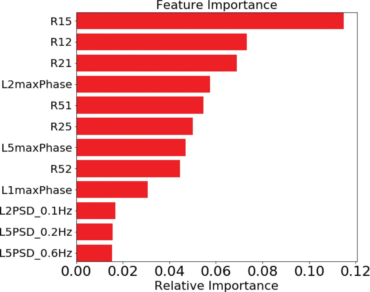
Illustration of feature importance of the random-forest algorithm. The top 12 most important features are presented. In this example, the random forest is trained using Feature Set #3 with triple-frequency signals.
The following notations are used in Figure 5:
Rij: The detrended phase ratio between Li and Lj carrier with a threshold on Lj
LimaxPhase: the maximum value of GPS Li PSD
LiPSD_mHz: the GPS Li PSD value at mHz
Figure 5 shows that the ratio between L1 and L5 with a threshold on L5 is the most important feature. This is reasonable because L1 and L5 have the greatest difference in carrier frequency, and thus lead to a better ratio separation between oscillator anomalies and scintillation. The L1 and L2 ratios are also important because the frequency difference between L1 and L2 is slightly smaller than the one between L1 and L5, but still comparable. The ratios of L2 and L5 are less important because these two frequency bands are closer to each other and hence show a smaller ratio separation.
The maximum values of the PSDs from three frequency bands (L1maxPhase, L2maxPhase, and L5maxPhase) are also important as shown in Figure 5. This is because it is the key indicator between phase disturbance and quiet time cases.
Finally, the PSD itself is less important compared to the ratios and maximum values of the PSD. This is reasonable because a single value at a specific frequency in the PSD fails to offer enough information for the classification. However, the entire PSD as a whole helps the classification task as its feature importance accumulates. These observations demonstrate that the max values of the PSD and ratios based on frequency dependence are essential features, which lead to a good detection performance.
3.3 Performance Comparison with Other ML Algorithms and the State-of-the-Art Detection Method
The random-forest algorithm performance is also compared with logistic regression, linear SVM, decision tree, neural network, and RBF (radial basis function) SVM, all using the same Feature Set #3 as input features. It is also compared to the state-of-the-art detection method presented by Liu and Morton (2020b). A brief summary of these methods is listed below:
Logistic Regression (Bishop, 2006) is a linear model that uses a logistic function to model the task. Logistic regression can only be applied for binary classification. To adopt it to our three-class classification setting, we took the so-called one-vs-one strategy by performing three pairs of binary classifications: oscillator anomalies vs. scintillation, scintillation vs. quiet time cases, and quiet time vs. oscillator anomalies. Three logistic functions are independently employed, wherein each is used to conduct the binary classification task for one pair. The final decision is made by the majority voting of these three logistic functions. In the event of a tie, it selects the class with the highest aggregate classification confidence by summing up the pair-wise classification confidence levels computed by the logistic function (Cournapeau, 2011).
Linear SVM (Bishop, 2006; Chang & Lin, 2011; Jiao et al., 2017; Liu & Morton, 2020b) is a method that uses a linear kernel for SVM. Its decision boundary is linear. It is also a binary classifier. The same one-vs-one strategy used in logistic regression is used.
A Decision Tree (Bishop, 2006; Quinlan, 1986) is a tree-like model that can handle multi-class classification tasks. As discussed in Section 2.1, the decision tree, itself, is a valid classifier. The drawback is that this method tends to overfit.
A Neural Network (Bishop, 2006) consists of a series of fully connected layers. It can deal with non-linearly separable problems and multi-class classification tasks.
RBF SVM (Bishop, 2006; Chang & Lin, 2011; Jiao et al., 2017; Liu & Morton, 2020b) is a method that uses a radial basis function (RBF) as the kernel. Its decision boundary can be non-linear. As a binary classifier, the one-vs-one strategy is employed.
SVM-RBF SVM (Liu & Morton, 2019, 2020a, 2020b) is a state-of-the-art ML-based oscillator anomaly detection process. To identify the oscillator anomaly, it involves two steps: in the first step, a linear SVM is proposed to detect a phase disturbance (Jiao et al., 2017a). Given the detected phase disturbance, an RBF SVM is then used to differentiate oscillator anomaly from scintillation. We shall refer to this two-stage approach as SVM-RBF SVM.
It should be noted that all algorithms presented (except SVM-RBF SVM) simplify the detection of oscillator anomalies into one step, where the differentiation of oscillator anomalies, scintillation, and quiet time samples is achieved through one classifier. In contrast, the detection of oscillator anomaly using SVM-RBF SVM involves two stages.
As shown in Table 3, logistic regression and linear SVM present the worst performance because these two linear algorithms fail to deal with non-linearly-separable problems. The decision tree also presents similar performance because it tends to overfit. The neural network exhibits comparable performance on dual-frequency signals and better performance on triple-frequency signals compared to the previous three algorithms. The reason could be that the neural network fails to capture the relationship when the frequency diversity is low.
Performance comparison between the random-forest algorithm, logistic regression, linear SVM, decision tree, neural network, RBF SVM, and SVM-RBF SVM. Ten different training/testing splits are used. The mean of the metrics is shown. FPR denotes false positive rate; TPR denotes true positive rate; PPV denotes positive predictive value. Dual and triple denotes dual- and triple-frequency signals.
RBF SVM and the random-forest algorithm show the best detection accuracy. The FPR and PPV of the random-forest algorithm is better while the TPR of the RBF SVM is better. This indicates that the random-forest method has a lower false alarm rate while the RBF SVM has lower missed detection probability. By taking both TPR and PPV into account, the F1 score of the random-forest method is slightly higher.
The performance of the SVM-RBF SVM from Liu and Morton (2020b) is also shown in Table 3. It is clear that random forest outperforms the SVM-RBF SVM for both dual- and triple-frequency signals. We should note here that the detection performance for the SVM-RBF SVM presented by Liu and Morton (2020b) is different from the ones presented in Table 3 in this paper. This is because the detection accuracy of 98.4% shown in Table 2 by Liu and Morton (2020b) refers to the accuracy of its Stage 2 performance, while in this paper, the detection accuracy of 93.3% refers to the combined performance of its Stages 1 and 2.
The SVM-RBF SVM employs PSD features in Stage 1 and ratio features in Stage 2, whereas the PSD and ratio features are combined into one stage in the random-forest method. This concatenation of PSD and ratio features in one stage potentially offers more information, and thus leads to better performance.
Comparable FPR and PPV are observed from these two methods while a large performance improvement for the random-forest algorithm is shown in TPR. This means that both methods exhibit very good performance in PPV, indicating that if an oscillator anomaly is detected, it has a very high probability of being a true oscillator anomaly.
However, the SVM-RBF SVM shows a poor TPR, indicating that the method has a higher missed detection probability. This could imply that poor phase disturbance detection in the first stage leads to a number of undetected oscillator anomalies, where these undetected oscillator anomalies could have similar PSDs to the quiet time samples. Thus, the features of the PSD fail to differentiate between them. This observation again demonstrates that the PSD and ratios between carriers offer distinctly different information.
4 DETECTION RESULTS
In this study, we applied the random-forest-based detection method to a database collected by our global GNSS monitoring network in 2017 and 2018, where Septentrio PolaRx5S receivers were deployed to obtain 100 Hz phase measurements (Jiao, 2017). It should be noted that the detection algorithm is trained on data collected from 2013–2016. This setup is to validate the general applicability of the algorithm to data that were not used in training. SVM-RBF SVM is also applied for the purpose of comparison. Station locations include Alaska, Greenland, South Korea, Puerto Rico, and Chile. The choice of these stations is based on the data availability, which is shown in Table 4.
Summary of data availability
All GPS Block IIRM and Block IIF satellites are processed by using the random-forest method with dual-frequency signals. As previously mentioned, differentiation between satellite and receiver oscillator anomalies is done by checking whether the same anomaly occurs on all satellites in view at the same time. The purpose of this section is to demonstrate the effectiveness of the random-forest detection method. A comprehensive characterization of satellite oscillator anomalies is currently underway and is the subject of a future publication.
We first use this database to compare the random-forest method with the SVM-RBF SVM. Here, the same database is also processed using the SVM-RBF SVM with dual-frequency signals. Table 5 shows the number of detected satellite oscillator anomalies for each method from each station. It is clear that the random-forest method is capable of detecting more anomalies compared to the SVM-RBF SVM. This observation supports our performance analysis in Section 3.3, wherein we suspected that a poor phase disturbance detection in SVM-RBF SVM may lead to undetected anomalies.
Comparison of station-wise statistics of detected satellite oscillator anomaly events on GPS Block IIRM and Block IIF satellites
Table 5 also demonstrates the capability of the random-forest algorithm on satellite oscillator anomaly detection. On average, 30–50 satellite oscillator anomaly events are detected by each station daily. The Alaska station has the highest average number of observations (49.6/day) and Puerto Rico and Chile have the lowest average number of observations (34.3/day). It should be noted that Table 3 shows that the TPRs of SVM-RBF SVM and the random-forest method are ~76% and ~95%, respectively, which shows ~20% difference on true positive rate (detection rate). However, as shown in Table 5, the number of detected events of random forest is ~10 times larger than the one of SVM-RBF SVM. The reasons that cause this discrepancy are as follows: To ensure a fair comparison in performance evaluation, the same data set (the data set with samples that are 30-second chunks) is used for the random-forest method and SVM-RBF SVM. This yields the TPRs in Table 3. In the detection results, the classifier in the first stage of SVM-RBF SVM is inherited from Jiao et al. (2017a) so the classifier is not re-trained as what we did in the performance evaluation. It was designed to detect scintillation and missed a large number of small satellite oscillator anomalies. As a result, the detection results of SVM-RBF SVM show a significantly smaller number of detected anomalies compared to the random-forest method, which are consistent with the numbers shown in Table 5 in Liu and Morton (2020b).
In the detection results, ~35 anomalies are detected from stations in South Korea and Chile per day. It should be noted that the data from these two stations are not used for training the detection method. This demonstrates that the detection method is generally applicable to stations at locations that were not included in the training.
In total, ~32,000 satellite oscillator anomalies are detected by the random-forest algorithm. In comparison, only 317 receiver oscillator anomalies are detected. To verify that the events detected by the random-forest algorithm are genuine satellite oscillator anomalies, 200 events were randomly selected from the detected anomalies and manually inspected. Among them, only three events were false positives, indicating a PPV of 98.5%. This PPV roughly matches the PPV (97.7%) of the random-forest method for dual-frequency signals in Table 3, indicating that the random-forest algorithm works as expected.
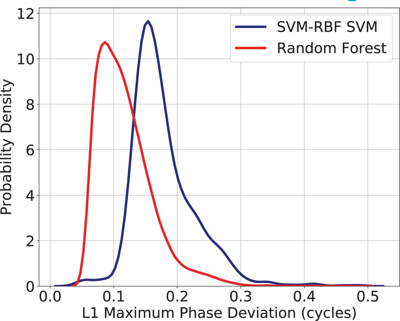
The comparison of the distributions of maximum phase deviation at L1 is shown in Figure 6, where the curves are obtained by the distribution fit to the histograms. The plot shows that the random-forest distribution shifts to the left of the SVM-RBF SVM distribution. This indicates that the random-forest algorithm detected many anomalies with smaller maximum phase deviations that are missed by SVM-RBF SVM. Figure 6 also shows that the most events detected by the random-forest method have a L1 maximum phase deviation below 0.4 cycles, although it also detects a few events that have larger L1 maximum phase deviations (above 0.4 cycles). In total, the random-forest method detects 32 large anomaly events, with 13, 12, 4, and 3 events from PRN 1, PRN 6, PRN 10, and PRN 26, respectively.

Comparison of the distributions of L1 maximum phase deviation between random forest and SVM-RBF SVM. The curves above are obtained by the distribution fit to the histograms
As mentioned in Section 2.3, a detected satellite oscillator anomaly event can be further confirmed if it is simultaneously observed by multiple stations. It should be noted that each anomaly event is independently detected by the random-forest method. If multiple detected anomaly events from the same satellite are simultaneously observed at different stations, they correspond to the same satellite oscillator anomaly. We process these detected events by grouping the events that correspond to the same satellite oscillator anomaly.
The results are shown in Table 6. There are 5,385 anomalies observed by two stations, 1,085 anomalies observed by three stations, and 5 anomalies that are simultaneously observed by four stations.
Satellite Oscillator Anomalies Observed by Multiple Stations in 2018. Stations include Greenland, Alaska, South Korea, and Puerto Rico.
One example of an anomaly observed by four stations is shown in Figure 7. Although different noises are present, the four stations show the same shape of the anomaly at the same time, confirming that the detected event is indeed a satellite oscillator anomaly, which again demonstrates the effectiveness of the random-forest method on satellite oscillator anomaly detection.

A satellite oscillator anomaly that is simultaneously observed by four stations (Alaska, South Korea, Greenland, and Puerto Rico). The anomaly occurred at 6:39 AM, on May 23, 2018 UTC for PRN 10, which is over Pacific Ocean, close to the US coast at that time
A histogram for each satellite’s average oscillator anomaly observations per visible day per station is shown in Figure 8. Here, a visible day refers to a 24-hour period during which the corresponding satellite is in view with elevation above 30 degrees at a station. Red PRN numbers refer to GPS Block IIRM and blue PRN numbers refer to GPS Block IIF. The PRNs are sorted by launch time (PRN 17 is the oldest satellite).

Satellite-wise average number of detected satellite oscillator anomaly events per visible day at each station. PRNs are sorted by launch time (PRN 17 is the oldest satellite). Red PRN numbers refer to GPS Block IIRM and blue PRN numbers refer to GPS Block IIF. The anomalies are detected by the random-forest algorithm.
It is apparent that most satellite oscillator anomaly events are from Block IIF satellites. In particular, the largest average number of events is observed in Alaska for PRN 10. On average, most Block IIF satellites show approximately 8–36 events per visible day per station. The exceptions are PRN 8 and PRN 24, where very few anomaly events were observed. We should note here that currently PRN 8 and PRN 24 use Cesium clocks while the rest of the PRNs in Block IIF use Rubidium clocks (Yang et al., 2019).
In contrast to Block IIF, all Block IIRM satellites observe very few anomaly events. Finally, the average number of anomalies per visible day does not increase with the age of the satellite, indicating that the aging factor does not have a clear correlation with the occurrence of anomalies.
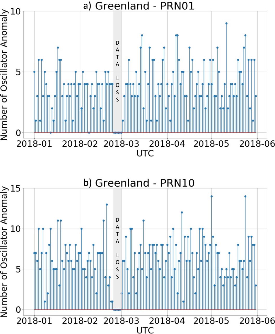
The time series of satellite oscillator anomaly daily occurrence is also investigated. Figure 9 shows the oscillator anomaly daily occurrence over Greenland from PRN 1 and 10. Random daily occurrence patterns are observed from both satellites. This indicates no periodic pattern is observed from detected oscillator anomaly events.

Satellite oscillator anomaly daily occurrence over Greenland. a) PRN 1; b) PRN 10. The anomalies are detected by the random-forest method.
In short, the random-forest method outperforms SVM-RBF SVM and shows its capability of automatically monitoring satellite oscillator anomaly events.
5 CONCLUSION AND FUTURE WORK
This paper demonstrates a machine-learning-based satellite oscillator anomaly detection method. It is based on a random-forest algorithm that uses input features containing the detrended carrier phase PSD and phase disturbance ratios from two carriers. The detection accuracies are 98.4% and 99.0% for dual- and triple-frequency signals, respectively.
The method outperforms linear SVM, logistic regression, decision tree, neural network, and RBF SVM. Compared to the state-of-the-art method SVM-RBF SVM, it not only simplifies the detection process but also shows better performance. Preliminary detection results demonstrate that the random-forest-based method can be employed in a global satellite oscillator anomaly monitoring system. The detection method also identifies ionospheric scintillation accurately, indicating that the method can also be applied to monitor scintillation.
The accurate detection performance shows the potential to apply this method in a global satellite oscillator anomaly monitoring system. In the future, the detection method will be applied to the data collected by our global GNSS monitoring network. A comprehensive global characterization of the satellite oscillator anomalies will be investigated. A series of explorations including the occurrence pattern and the behavior for different GPS satellites will be conducted. In addition, limited availability of the high rate (100 Hz) GPS receivers may prohibit a comprehensive global characterization. In the future, an investigation of whether low-rate GNSS receivers (1 Hz) from a public GNSS network is capable of detecting satellite oscillator anomalies by using the proposed method will be conducted. Finally, the current detection method has limitations on detecting satellite oscillator anomalies outside the frequency range from 0.1 Hz to 2 Hz due to the feature extraction design. The extension of satellite oscillator anomaly detection to higher frequencies will be conducted, which will also involve interference detection.
HOW TO CITE THIS ARTICLE
Liu, Y. & Morton, Y. T. J. (2022). Improved automatic detection of GPS satellite oscillator anomaly using a machine learning algorithm. NAVIGATION, 69(1). https://doi.org/10.33012/navi.500
ACKNOWLEDGMENTS
This work is supported by the Space Weather Technology, Research, and Education Center (SWxTREK), the University of Colorado at Boulder, and a contract from Lockheed Martin. The authors are grateful to Mr. Ian Collett for his valuable comments and suggestions on the manuscript. The data used in this study was collected at the global ionospheric scintillation monitoring network established by the Satellite Navigation and Sensing (SeNSe) Lab at the University of Colorado Boulder.
- Received August 9, 2020.
- Revision received August 13, 2021.
- Accepted August 14, 2021.
- © 2022 Institute of Navigation
This is an open access article under the terms of the Creative Commons Attribution License, which permits use, distribution and reproduction in any medium, provided the original work is properly cited.


Jump to section
Related Articles
Cited By...
- No citing articles found.