

Abstract
High-precision positioning methods have drawn great attention in recent years due to the rapid development of smart vehicles as well as automatics driving technology. The Real-Time Kinematic (RTK) technique is a mature tool to achieve centimeter-level positioning accuracy in open-sky areas. However, the users who drive under dense urban conditions are always confronted with harsh global navigation satellite system (GNSS) environments. Skyscrapers and overpasses block the signals and reduce the number of visible satellites, making it difficult to achieve continuous and precise positioning. Considering that the road is relatively smooth in most urban areas, vehicles are expected to travel on the same plane when they are close to each other. The road plane information is a promising candidate to enhance the performance of the RTK method in constrained environments. In this paper, we propose a plane-constrained RTK (PCRTK) method using the positioning information from cooperative vehicles. In a vehicle-to-vehicle (V2V) network, the positions of cooperative vehicles are used to fit a road plane for the target vehicle. The parameters of the plane fitting are treated as new measurements to enhance the performance of the float estimator. The relationship between the plane parameters and the state of the estimator is derived in our study. To validate the performance of the proposed method, several experiments with a four-vehicle fleet were carried out in open-sky areas and dense urban areas in Beijing, China. Simulations and experimental results show that the proposed method can take advantage of the plane constraint and obtain more accurate positioning results compared to the traditional RTK method.
1 INSTRUCTION
Global navigation satellite systems (GNSS) have been widely employed in vehicular applications to conduct real-time position estimation (Dabove, 2019; Du & Barth, 2008). One of the most competitive and promising positioning methods, the Real-Time Kinematic (RTK) technique (Hofmann-Wellenhof et al., 2001), is feasible to provide centimeter-level positioning accuracy once carrier-phase ambiguities have been correctly resolved. However, frequent signal blockages caused by skyscrapers and overpasses lead to degradation in satellite visibility (Alam & Dempster, 2013). In a harsh environment, the positioning accuracy of the RTK method may decrease significantly, leading to unacceptable positioning errors for some safety-critical vehicular applications (Alam et al., 2012; MacGougan et al., 2010).
To achieve reliable and precise positioning in urban scenarios, a feasible approach is to extend the RTK method by fusing other positioning sensors (Zhao et al., 2016). Lassoued et al. (2016) proposed a tightly coupled integrated system using inertial navigation system (INS) and GNSS data, which realized robust positioning in various urban environments. Similarly, Qian et al. (2020) proposed a cooperative RTK algorithm by jointly using INS and light detection and ranging (lidar) data, which achieved a higher fixed rate and position accuracy compared to the traditional RTK method. Xiong et al. (2020) integrated ultra-wideband (UWB) sensors into the RTK method to improve the robustness of positioning. However, these methods require additional and expensive sensors to obtain accurate sensing information, which is inapplicable to low-cost vehicles (hereinafter referred to as common vehicles). Common vehicles and sensor-rich vehicles coexist in current traffic scenarios (Li et al., 2020). How to improve the positioning performance of common vehicles is still worth studying.
Owing to the fast development in the field of inter-vehicle communication (Zhang et al., 2018), vehicles equipped with communication devices are able to share navigation data with each other (Hu et al., 2021). The cooperative positioning (CP) method based on vehicle-to-vehicle (V2V) communication is a promising approach to enhance the positioning accuracy and reliability of common vehicles (Xiong et al., 2020; Song et al., 2020; Xiong et al., 2019). The theoretical features of achievable performance for CP have been deduced by Penna et al. (2010) and Schloemann and Buehrer (2015). Alam and Dempster (2013) discussed the feasibility of conventional and modern CP systems in vehicular applications. Inspired by their studies, we previously proposed a cooperative positioning algorithm that combined the benefits of the RTK method and the CP method (Zhuang et al., 2021). The accuracy of float solutions can be improved by fusing GNSS observations from neighboring vehicles. Thus, a higher ambiguity fixed rate can be achieved compared to the conventional RTK method. However, the computational load would be relatively high because additional ambiguities between the ego vehicle and cooperative vehicles must first be resolved.
As many researchers focus on the integration of cooperative GNSS measurements, some sensor-free environmental features that can also improve the positioning performance are seldom considered in CP methods (Alam & Dempster, 2013). In urban scenarios, the road conditions are generally good and the roads are relatively smooth (Múčka, 2017), which means neighboring vehicles are usually traveling on the same plane that the ego vehicle is located. Therefore, we can use the plane information obtained from cooperative vehicles as new measurements to constrain the float estimator of the traditional RTK method.
In this paper, we propose a plane-constrained RTK (PCRTK) method using positioning solutions from cooperative vehicles. By collecting positioning data of cooperative vehicles traveling on the same road, we derive a plane equation and use the parameters of the plane equation to constrain the float estimator. The main contributions of our work include the design of a plane construction method using the positioning solutions shared by cooperative vehicles and the derivation of a float estimator based on an adaptive Kalman filter that fuses the plane parameters with GNSS observations. We carried out several field tests involving four vehicles to collect real data to verify the proposed method. Numerical simulations and experimental results validate the feasibility and superiority of our method.
The paper is organized as follows: In Section 2, we introduce the construction of the height plane; in Section 3, we describe the main procedure of the PCRTK method; then, the proposed method is validated by several simulations and experiments in Section 4 and Section 5; discussions on the limits of the proposed method are presented in Section 6; and finally, we conclude our work in Section 7.
2 THE CONSTRUCTION OF THE HEIGHT PLANE
Consider the following scenario: Vehicles traveling on a smooth road can share their positioning data and the distance of their GNSS antennas from the ground through inter-vehicle communications. A vehicle can receive the data and then use them to fit a plane where the neighboring vehicles are traveling. To make it easier to understand the process of plane fitting, we define a target vehicle in this section and the others are regarded as cooperative vehicles. The process of plane construction can be divided into two parts: the construction of the road plane and the construction of the antenna height plane.
A GNSS antenna is generally placed on the roof of a vehicle. The height of a vehicle is generally different, which is determined by their brands. If the plane is constructed using the positions of the antennas directly, larger errors are inevitable for fitting the plane where the vehicles are truly located. In this case, the positions of the target vehicle are likely to incline to a faulty plane. Therefore, a road plane is first constructed by removing the height of the antennas of the vehicles. Then, we introduce the height of the antennas into the plane again. In this way, a plane expression that constrains the positions of the vehicles can be obtained.
Generally, the Earth-centered, Earth-fixed (ECEF) coordinate system is used. To deal with the height information of vehicles, the coordinate system is converted from ECEF to the local Cartesian coordinate system (East-North-Up or ENU) through an S matrix. Then, the baseline  between the position of a vehicle cast to the road plane and the reference station can be expressed as:
 1
1
where bi,k represents the baseline between the cooperative vehicle i and the reference station at the k-th epoch and hi is the antenna height of vehicle i. After eliminating the influence of vehicle height, we add the location of the reference station bo and calculate a new conversion matrix S′ from the projection of the vehicle on the road to the center of the Earth, and then convert the ENU coordinate system back to ECEF again:
 2
2
Relative positions are used rather than absolute ones, as it is more convenient for us to introduce the plane constraint into the float estimator.
According to Equation (2), a point set  can be obtained at epoch k. Only the data of one epoch may not be enough for fitting a plane. In our study, we selected the data of five consecutive epochs closest to the current time to fit a plane. The set for fitting a plane is defined as V′ in this paper. We, by default, utilized all the available positioning solutions in V′ to fit the plane. The least-squares method (Hurt & Colwell, 1980) was used to fit the plane α, whose distance to these positioning solutions was minimal:
 3
3
 4
4
where mean(·) is the mean function, SVD(·) is the singular value decomposition (SVD) function, and U, S, V are the corresponding matrices.
After the SVD, the eigenvector corresponding to the minimum singular value is the normal vector of the plane, which is expressed as:
 5
5
where end represents the index of the minimum singular value. Meanwhile, the normal vectors also satisfy the following relationship:
 6
6
The constant term can be expressed as:
 7
7
Then, the expression of the road plane is defined as:
 8
8
where x, y, z are the three-dimensional coordinates under the ECEF frame.
After the construction of the road plane, we can obtain the plane of the target vehicle by translating the road plane up by the height of the target vehicle ho as:
 9
9
where:
 10
10
where the left side of Equation (10) does not have the sign of absolute value since the direction of translation is known. This equation can be further simplified according to Equation (6) as:
 11
11
It is worth noting that the premise of using the plane constraint is that the vehicles are traveling on the same plane and the positioning solutions used to fit the planes are accurate enough. Therefore, it is necessary to check whether the positioning solutions used for fitting the planes meet this requirement before introducing the plane constraint into our method. In this paper, a plane detection procedure was conducted by comparing the residual of plane fitting with a preset threshold.
In our study, we focus on the average value of the residuals in fitting a plane, which is calculated by:
 12
12
where:
 13
13
Here, N is the number of cooperative vehicles. It is recommended that at least two vehicles participate in fitting the plane and they are best traveling in different lanes. In this way, the plane can be constructed from the perspective of geometry. kstart and kend represent the starting epoch and the end epoch for selecting positioning results. di,k is the distance between the position  and the fitted plane. If all the cooperative vehicles travel on the same plane and their positions are accurate enough, the residual of plane fitting would be small, which is regarded as a normal case in our study. Otherwise, the positions of some cooperative vehicles would be far away from the plane and the residual would be larger, which is regarded as a faulty case. Therefore, whether the positioning solutions used for plane fitting belong to the same plane or not can be determined by:
 14
14
where Tfitting is the threshold for plane detection. The value of the threshold depends on the distribution of the residuals of plane fitting and the false alarm rate. In our study, precise positioning results collected in a flat and open-sky area are used to calculate the distribution function and the threshold. The details on how to use the distribution of the residuals and false alarm rate to calculate the threshold are given in Section 4. If the plane fitting cannot pass detection, an iterative procedure is implemented to remove the positioning result with the largest residual in plane fitting one by one, which is similar to the fault exclusion procedure in the Receiver Autonomous Integrity Monitoring (RAIM) method (Hsu et al., 2017). The removal procedure is repeated until the plane detection has passed or the number of remaining positioning results used to fit the plane is less than a pre-set value, which is set to 10 in this paper.
The positions of the target vehicle can be constrained by this plane. Based on the constructed plane, a Kalman filter is employed to calculate float solutions. However, in high dynamic scenarios, multipath, non-line-of-sight (NLOS), and other types of interference make it challenging to determine the noise covariance matrix Q and R correctly, which may greatly affect the accuracy of estimation (Liao et al., 2017). Thus, we employ an adaptive Kalman filter to update the noise matrix and improve the stability of the estimator.
3 PLANE-CONSTRAINED RTK METHOD
The architecture of the proposed method is illustrated in Figure 1. In the first stage, the vehicle plane is constructed by the positioning results of cooperative vehicles. Then, an adaptive Kalman filter estimator is used to resolve the float solutions. Finally, the float solutions are sent to an integer ambiguity resolution model to calculate the fixed solutions. The final solutions are saved and used for the plane construction of other vehicles in the next epoch.
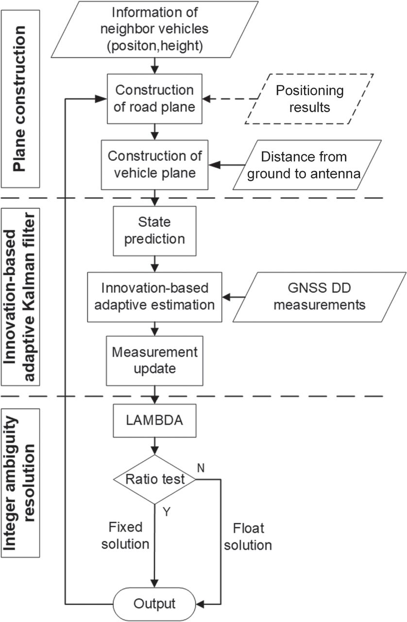
Architecture of plane-constrained RTK method
3.1 GNSS Double-Differenced (DD) Observation Model
Double-differenced (DD) pseudorange and carrier-phase observations can be expressed as:
 15
15
 16
16
where ∇Δ represents the DD calculation. ρ and ϕ are the original observation of pseudorange and carrier phase, respectively. p is the actual distance between the satellite and receiver. λ and N are the wavelength and integer ambiguity of carrier phase. The subscript rb denotes the difference between the corresponding terms of rover and base, while the superscript ij denotes the difference between the j-th satellites and the i-th (reference) satellite. As the baseline between the vehicles and base station is usually short, the ionospheric and troposphere delay is neglectable in DD equations.
To further excavate the baseline vector from the DD equations, we linearize  and save the first-order term:
 17
17
where  represents the unit line-of-sight vector from the receiver to satellite and bur represents the baseline vector.
3.2 Float Estimator Based on Adaptive Kalman Filters
In our proposed method, the state vector is defined as:
 18
18
where bur, vur, and aur are the baseline, velocity, and acceleration vectors between the rover and base station.  represents the DD float ambiguity vector.
The system model is defined as:
 19
19
 20
20
where Xk,k−1 is the current state vector and Xk−1 is its previous state vector. F represents the system state transition matrix and ωk is the process noise at epoch k while Q is its covariance matrix. Pk,k−1 is the estimated covariance matrix of the previous epoch.
The state transition matrix is written as:
 21
21
 22
22
 23
23
where τ is the filtering period and Im is the identity matrix with size m. The observation vector is defined as:
 24
24
where  and
and  are the DD pseudorange and carrier-phase observations and
  is the constant coefficient in Equation (9). Then, the observation model is defined as:
 25
25
where Zk is the current observation vector, H is the observation matrix, and vk is the observation noise, while R is its covariance matrix.
The observation matrix is written as:
 26
26
where:
 27
27
 28
28
 29
29
where PA, PB, and PC are the corresponding coefficients in Equation (9).
The basic equations of the Kalman filter are written as:
 30
30
 31
31
 32
32
where Kk represents the Kalman gain, Xk is the posterior state vector, and Pk is the estimated covariance matrix.
In a general Kalman filter estimator, the process noise matrix Q and the observation noise matrix R are preset values. Thus, the influence of the surrounding environments has been ignored. In order to obtain a more accurate noise matrix, we adopted the innovation-based adaptive Kalman filter method proposed by Mohamed and Schwarz (1999) to update the noise matrix at each epoch. If Q and R are estimated simultaneously, the estimator can be misled by their relation and even diverge. To avoid this problem, a feasible solution is to estimate just one of them instead of both of them. Therefore, we only estimate the update measurement noise matrix R while the system noise matrix Q is regarded as a constant matrix.
The elements of the innovation-based sequence are defined as the difference between observations and prediction values, which is written as:
 33
33
The variance of innovation-based sequence is defined as:
 34
34
In practical situations, it can be calculated by:
 35
35
 36
36
where k represents the current epoch and L is the window size of the innovation-based sequence. Since divergence may occur if the number of equations required to estimate the unknown adaptive parameters is smaller than the number of unknowns, themselves, a window size larger than the number of update measurements is needed when adapting R and a window size larger than the number of filter states is required when adapting Q.
The theoretical value of such variance is defined as:
 37
37
Let  , then Q and R matrices can be estimated by:
 38
38
 39
39
Although we give the derivation of both Q and R, only the update measurement noise matrix R is estimated while the system noise matrix Q is regarded as a constant matrix.
It worth noting that if Q is not positive semi-definite or R is not positive definite, the estimator may diverge. This phenomenon occasionally occurs in severe multipath-affected areas. If R is not positive definite or Q is not positive semi-definite, we use a constant R or Q instead. The output of this filter is the float baselines and float ambiguities. The next step is to convert the float carrier-phase ambiguities into integer carrier-phase ambiguities.
3.3 Integer Ambiguity Resolution
After the Kalman filter, the float state vector  and the float ambiguity vector
  can be obtained. To fix the DD float ambiguities, the common least-squared ambiguity decorrelation (LAMBDA) method is used (Teunissen, 1995). By searching over a set of integer grid points near the float resolution, LAMBDA finds some candidates that satisfy the equation:
 40
40
where  is estimated covariance matrix for float DD ambiguities. χ2 is the size of searching space. After the searching step, a ratio test is employed as the acceptance test:
 41
41
where N1st and N2nd are the best and second-best candidates, respectively. ξ is the threshold of ratio test, which is set to 3.
When the best candidate passes the ratio test, we can get the fixed solutions by updating  as:
as:
 42
42
where  is the estimated covariance matrix between the float state vector and DD ambiguity vector and N is the fix ambiguity vector.
In our study, we adopt an instantaneous mode rather than a fix-and-hold mode for handling the integer ambiguity resolution. This means that the integers are resolved in each epoch independently and the integer fixes are not maintained. At each epoch, we try to fix all the ambiguities rather than just some part of them.
3.4 Extending the PCRTK Method to a Cooperative Network
In the above subsections, we focus on how to apply the plane-constrained method to a specific vehicle. Only the target vehicle is assumed to conduct the proposed PCRTK method, while the others are regarded as information providers that calculate their positions by using a non-cooperative method. In this section, we discuss how to apply the proposed method to each vehicle in a cooperative network.
Figure 2 depicts the structure of a cooperative network involving a total of M vehicles. All the vehicles in this network belong to peer nodes, which means these vehicles will share information between each other and conduct the same positioning algorithm. bi,k represents the positioning results of vehicle i at epoch k. hi denotes the distance from the GNSS antenna of vehicle i to the ground, which is a fixed value measured for each vehicle. We assume that all the vehicles have obtained their positioning results of epoch k.
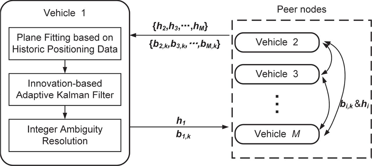
The extension of the plane-constrained method to a cooperative network
Taking Vehicle i as an example, it will broadcast its own positioning data bi,k of epoch k to the others and receive the positioning data  from peer nodes simultaneously. The positioning results of peer nodes from epoch k − Nfitting + 1 to k − 1 are also stored by Vehicle i, where Nfitting is the number of positioning solutions provided by each vehicle for fitting the planes. Vehicle i utilizes these positioning solutions to fit a plane, and calculates its position of epoch k + 1 using the PCRTK method. Once Vehicle i obtains its position solution of epoch k + 1, it will broadcast the latest positioning solution to the others and then receive new positioning solutions from peer nodes for calculating its own position at the next epoch.
The same process can be applied to the other vehicles in this network. In this way, all the vehicles in this network can benefit from the proposed method. Since the proposed method is distributed and adopts the time series of positioning solutions to fit the planes, the demand for time delays is reduced compared to other ranging-based cooperative positioning methods.
It is worth noting that the resulting error correlation is inevitable due to the feedback from the other receivers in the network. If the PCRTK position solution of vehicle A suffers from a large error, vehicle B cooperating with vehicle A will be affected when fitting the plane without any fault exclusion. Then the position solution of vehicle B will be contaminated and affect vehicle A in turn, resulting in error correlation. Fortunately, the plane detection algorithm proposed in Section 2 can effectively reduce the influence of the resulting error correlation. An iterative procedure is implemented to remove the outliers in plane fitting one by one. In this way, we can avoid utilizing position solutions with large errors to fit the plane to ensure the reliability of the plane constraint and the stability of PCRTK method.
4 SIMULATIONS BASED ON GNSS DATA COLLECTED IN OPEN-SKY AREAS
To evaluate the feasibility of the proposed method, simulation results are given in this section. These simulations were based on GNSS data collected in a ground vehicle test, which was conducted in open-sky areas in Beijing, China. The road was extremely smooth with few bumps and there were few cars traveling in the test areas, so we could drive the test vehicles in different formations.
Figure 3 presents the test route in which the red star denotes the location of the reference station. Four vehicles (referred to as V1, V2, V3, and V4, respectively) were involved in the test and traveled along the same route during the test. Each car was equipped with a GNSS receiver to collect GNSS measurements. In this test, V1 was equipped with a GNSS receiver named M300, which belongs to a consumer-grade receiver. V2, V3, and V4 were equipped with NovAtel OEM628, OEM7500, and Trimble BD992 receivers, respectively. The data of GPS L1/L2 and BeiDou B1/B2 were collected at 1 Hz during the test. The distance of the GNSS antennas from the ground was measured for each vehicle before the test.

The test route in open-sky areas
The INS data were also collected by each vehicle as an input to the post-processing system (NovAtel Inertial Explorer). The raw GNSS observations of all-in-view satellites together with INS data and the precisely known location of the reference station were processed using NovAtel Inertial Explorer to calculate the absolute reference solutions for each vehicle. Since all the GNSS data were collected under good observation conditions, the horizontal root-mean-square error (RMSE) of the reference solutions could reach 0.01 m using RTK corrections under standard vehicle dynamics.
The sky plot of visible satellites observed by the reference station is shown in Figure 4. The initial G denotes GPS satellites and C denotes BeiDou satellites. The average number of satellites observed by the reference receiver was about eight for GPS and 15 for BeiDou. To simulate signal blockages in urban areas, the measurements of the satellites whose elevation angles were less than 45 degrees were removed from the positioning process of both the proposed method and traditional RTK method in the following simulations.
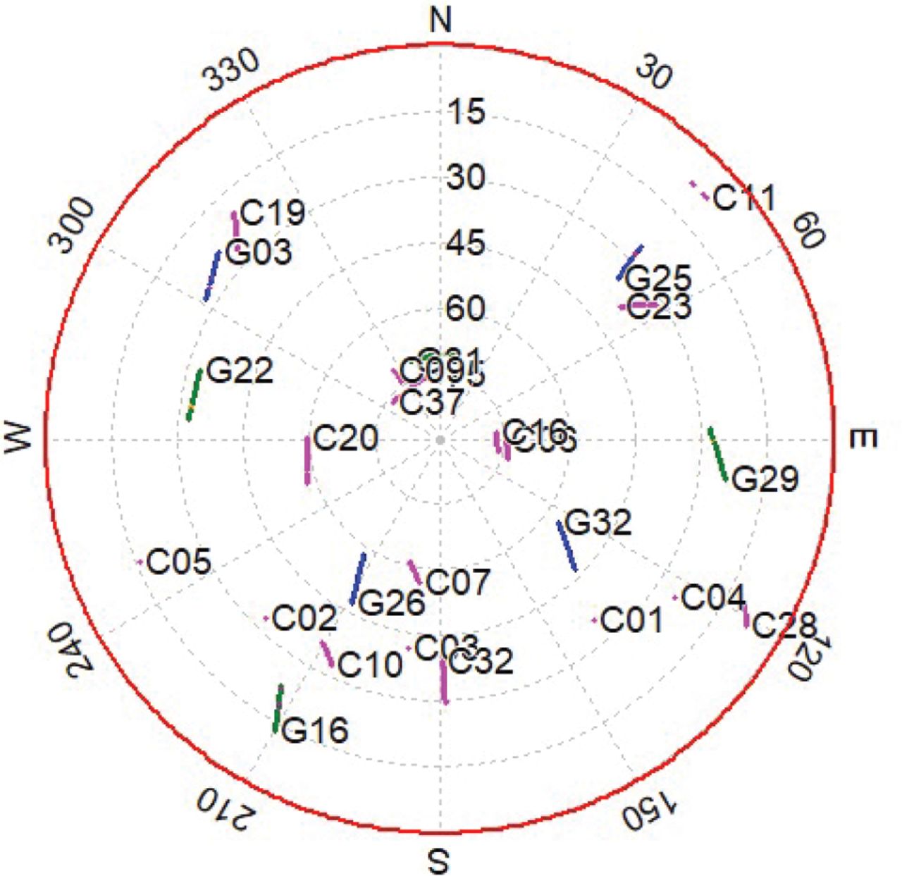
The sky plot of visible satellites received by the reference station during the test
4.1 Simulations on Plane Uncertainty
We imposed a constraint on the float estimator of the traditional RTK method by introducing a plane in which the vehicles would be traveling. The accuracy of this plane determines the performance of the proposed method. Therefore, the influence of plane uncertainty on the performance gain for the PCRTK method is analyzed in this subsection.
Since the plane is constructed using the positioning results of cooperative vehicles, the precision of the positioning results provided by these cooperative vehicles would definitely affect the uncertainty of the constructed plane and determine the benefit of using our method. To verify that the proposed method can benefit from the constraint of an accurate plane, we first adopted the reference solutions of the test vehicles to construct the planes and conduct the PCRTK method. Since the post-processed reference solutions are extremely precise and the vehicles were traveling on a flat road, the constructed planes would be quite accurate and the proposed method was expected to show its best performance in this case.
Considering that the vehicles can be treated as peer nodes and all the vehicles traveled under the same conditions, we only take Vehicle 4 (V4) as an example in this section. Figure 5 depicts the positioning errors’ cumulative distribution function (CDF) of PCRTK for V4 in the case that the plane was constructed using the reference solutions of cooperative vehicles. To make a comparison, the positioning errors of traditional RTK using the same data are also presented in this figure. Both PCRTK and RTK solutions were computed with a 45-degree mask angle to simulate signal blockages. Compared to the traditional RTK method, the proposed method shows an improvement in positioning accuracy. The proportion of positioning errors less than 1 m was 88.48% for the RTK method, rising to 96.76% for the proposed method. The plane constraints can be treated as additional measurements, which make a great contribution to the improvement in positioning accuracy.

The positioning performance of PCRTK for V4 in the case that the plane was constructed using reference solutions of cooperative vehicles
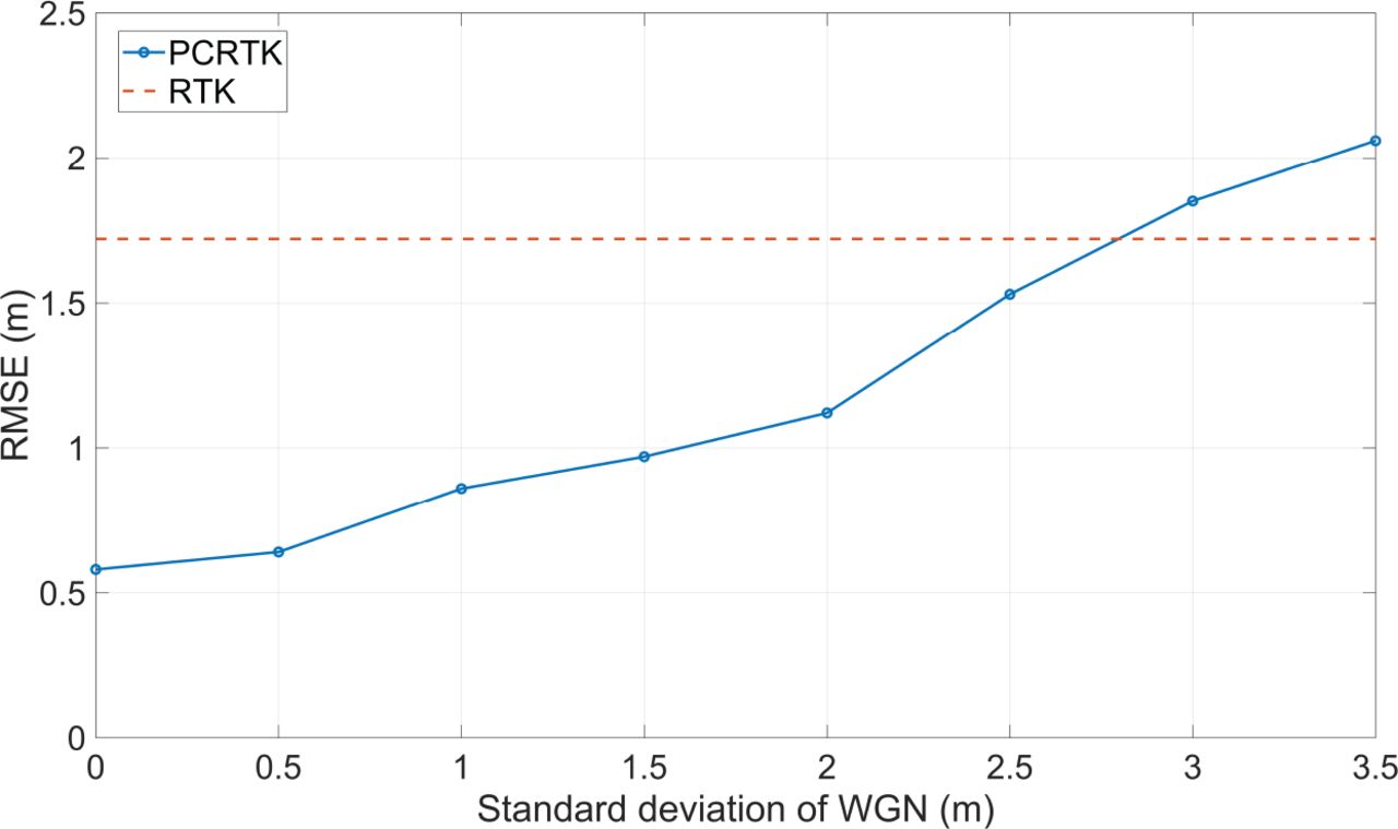
To simulate the uncertainty of the constructed planes, white Gaussian noise (WGN) with various standard deviations was added to the reference solutions of the test vehicles when we constructed the planes. More specifically, the WGN with various standard deviations was added to the three directions of reference solutions in ENU coordinates. In simulations, the standard deviation of the WGN ranged from 0 m to 3.5 m at intervals of 0.5 m. Figure 6 shows the RMSE of the PCRTK method for V4 in which the plane was constructed using reference solutions contaminated by WGN with various standard deviations. For comparison, the RMSE of traditional RTK is also marked in this figure, which is equal to 1.72 m.

The RMSE of the PCRTK method for V4 in the case that the plane was constructed using reference solutions contaminated by WGN with various standard deviations
The proposed method saw an upward trend in RMSE when the standard deviation increased from 0 m to 3.5 m, with the figure climbing from 0.58 m to 2.06 m. The reason for the degradation of positioning accuracy is that the inaccurate positioning solution used for constructing the plane resulted in an increased uncertainty of the constructed plane. If the plane parameters are treated as additional measurements in the float estimator, the increased uncertainty of the plane means an increase in observation noise. The magnitude of plane uncertainty can be reflected by the residuals of plane fitting, which was introduced in Equation (12). Figure 7 depicts the mean residuals of plane fitting when we introduced WGN with various standard deviations to reference solutions. It can be seen that the mean residuals of plane fitting increase with the growth of standard deviation.

The mean residuals of plane fitting in the case that the plane was constructed using reference solutions contaminated by WGN with various standard deviations
Since the positioning solutions provided by cooperative vehicles may not be accurate enough and we cannot rule out the possibility that vehicles travel on different planes, the method of selecting an appropriate threshold for constraining the plane uncertainty is extremely important. It worth noting that the RMSE of the proposed method is larger than the traditional RTK method when the standard deviation of the WGN added to reference solutions is greater than 3 m, which can be found in Figure 6. To ensure that the proposed method can benefit from the constraint of the plane, it is better to set a threshold for plane fitting, which was originally mentioned in Section 2. The threshold can be set according to the distribution of the residuals of plane fitting and a false alarm rate. We recorded the residuals of plane fitting in the case that WGN with a standard deviation of 2.5 m was introduced into the reference solutions. Since the RMSE of the PCRTK method was still lower than the RTK method in the case of a standard deviation of 2.5 m, the distribution of the residuals in this case was selected to calculate the threshold. Figure 8 presents the residuals of plane fitting in the case that WGN with a standard deviation of 2.5 m is added to the reference solutions. In our study, the false alarm rate was set to 1%. The final threshold was set to 2.6 m, which is used in the following simulations.

The residuals of plane fitting in the case that WGN with a standard deviation of 2.5 m is added to the reference solution
4.2 Performance of Extending PCRTK Method to a Cooperative Network
In Section 3, we introduced how to extend the PCRTK method to a cooperative network. If the cooperative vehicles of a vehicle also use the PCRTK method rather than non-cooperative methods such as traditional RTK, this vehicle would be expected to obtain more accurate positioning results since the positioning results used to fit the planes would be more accurate. To verify the benefit of extending the proposed method to a cooperative network, we make a comparison between the positioning results with and without access to a cooperative network. Taking V4 as an example, all the cooperative vehicles would adopt the traditional RTK method in the case that they are without access to a cooperative network, while the PCRTK method would be used by all the cooperative vehicles in the case that a cooperative network was available.
Table 1 gives the statistical results of V4 for the PCRTK method with and without cooperative network access. The results of the traditional RTK method are also given in this table so that we are able to see if the proposed method could benefit from the constructed planes in two cases. CEP95 represents the circular error at probability of 95%. It can be seen that the proposed method shows better positioning performance than the traditional RTK method whether the cooperative network was used or not. Compared to the case without a cooperative network, the PCRTK method with a cooperative network shows a drop in positioning errors, with the figure of RMSE decreasing from 1.01 m to 0.63 m. The improvement in positioning accuracy can be attributed to the improved precision of plane fitting. When the cooperative vehicles also use the PCRTK method, it is feasible to provide a more accurate positioning solution for V4 to fit the plane. The reason that CEP95 and RMSE cannot reach centimeter-level accuracy is that there are still some float solutions with relatively large errors. Therefore, it is difficult to achieve centimeter-level positioning accuracy overall.
Horizontal Position Statistics of V4 for PCRTK Method With and Without Cooperative Network
Since we verified the benefit of cooperative networks, we adopted the PCRTK method with a cooperative network in the following simulations and experiments. This means that all the vehicles utilized the proposed method to calculate their positions simultaneously.
4.3 Comparisons Between Different Formations
During the experiment, we attempted to drive the vehicles in different formations to evaluate the performance of the proposed method. Four kinds of formations were considered in the experiment that are shown in Figure 9. Since Vehicle 4 was used in the previous simulations, we also take V4 as an example in this section. The green represents V4 and the blue denotes the other vehicles.

The driving formations during the experiment
Table 2 gives the statistical results for V4 under different driving formations. It can be seen that the proposed method with formation (a) shows the worst positioning performance. Theoretically, points on the same line cannot be used to fit a specific plane. However, the positions of GNSS antennas are unlikely to keep a line even if the vehicles were traveling in a line. Therefore, the positioning results can also be used to fit the planes. In this case, a slight increase in the errors of the provided positioning solution might result in a great uncertainty of the constructed plane. Since the plane was constructed inaccurately, the positioning accuracy for formation (a) was also degraded. As for the cases of formations (b), (c), and (d), the proposed method shows similar positioning performance. The results of formation (b) show the best performance among these four cases because the vehicles traveled in formation (b) had better geometric distribution. The constructed plane was, thus, more accurate and reliable in this case.
Horizontal Position Statistics of V4 for the PCRTK Method in Different Formations
5 GROUND VEHICLE TEST IN DEGRADED ENVIRONMENTS
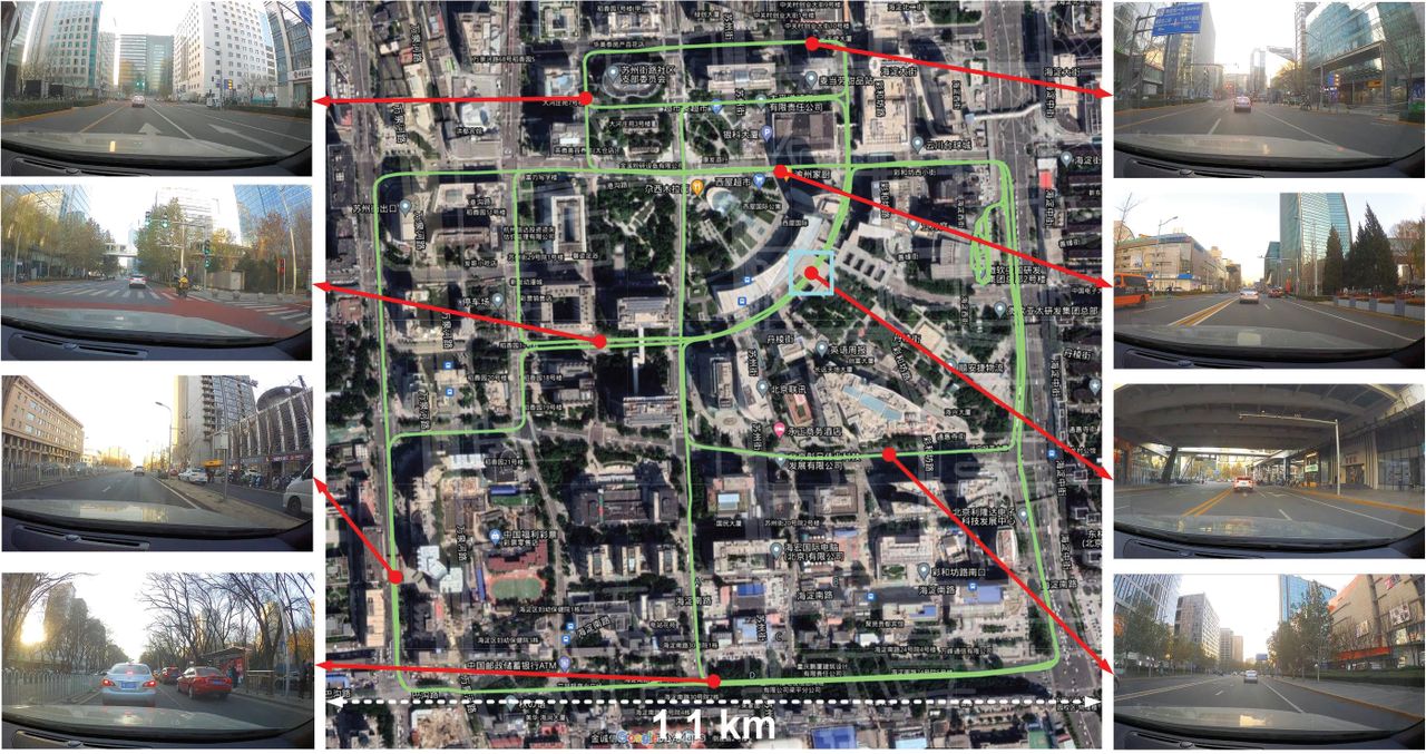
To evaluate the performance of the proposed method under degraded environments, several dynamic experiments were carried out in Zhongguancun E-park in Beijing, China, on the November 24, 2021. The test routes are depicted in Figure 10. A reference station with exact positioning was set in an open-sky area within 2 kilometers of the test routes to collect raw observations for differential GNSS. Four vehicles (also referred to as V1, V2, V3, and V4) traveled along the same routes in the experimental areas where high-rise buildings strongly challenge GNSS-based positioning performance.

The experimental routes in Zhongguancun E-park
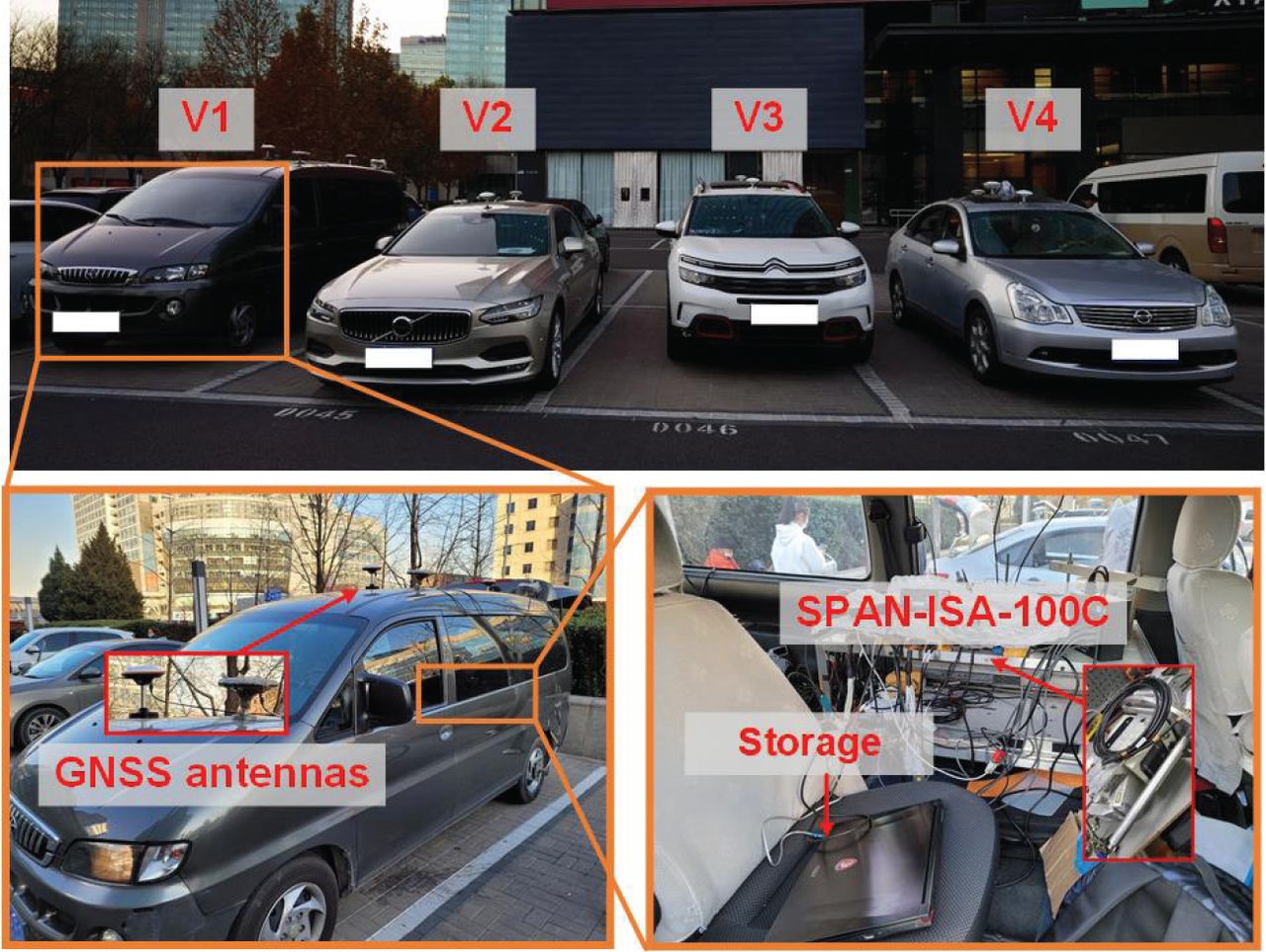
During the experiments, V1 was equipped with a NovAtel SPAN-ISA-100C integrated navigation system as shown in Figure 11. The other three vehicles were also equipped with an integrated navigation system named NPOS220, which consisted of a NovAtel OEM7500 receiver and an EPSON G320N inertial measurement unit (IMU). The collected raw GNSS measurements, together with IMU data of the vehicles, were sent to the post-processing software NovAtel Inertial Explorer to calculate the reference solution for each vehicle using RTK corrections. Only GNSS data were used to analyze the positioning performance of the proposed method and the control group.

The test vehicles participating in the experiments
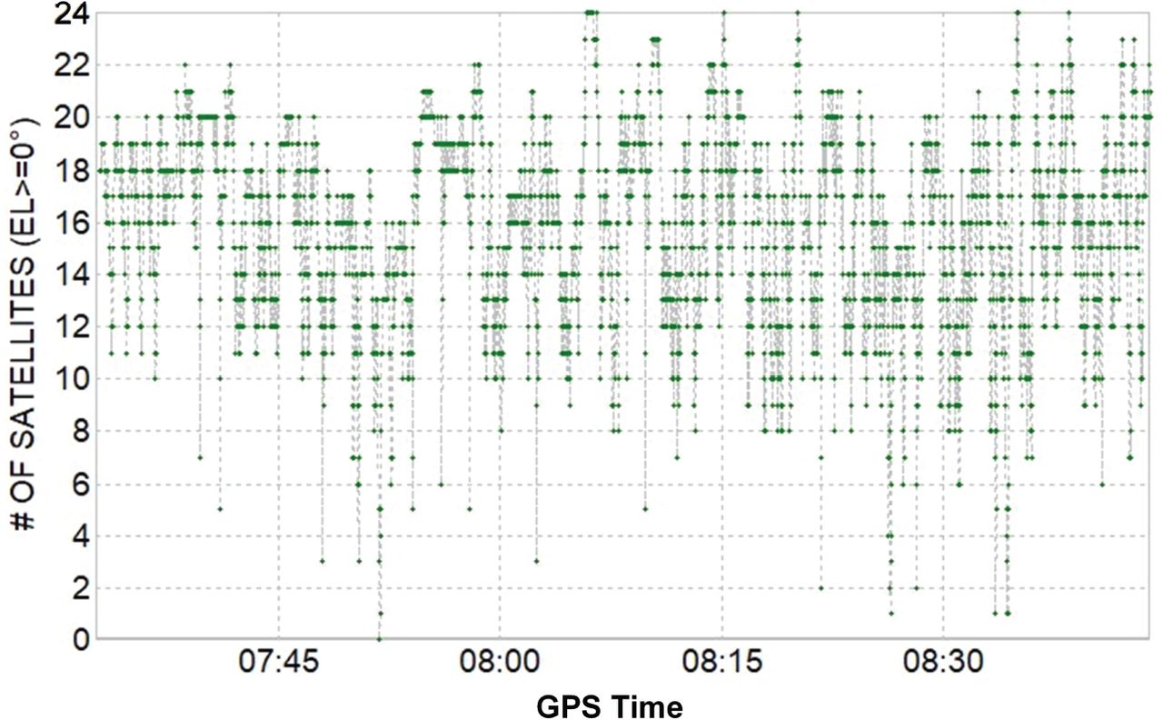
Figure 12 presents the satellite visibility of V4 during the experiments; the initial G denotes GPS satellites, the initial J represents Quasi-Zenith Satellite System (QZSS) satellites, and the initial C indicates BeiDou satellites. The green points represent the epochs when L1/2 or B1/2 could be received. The yellow points denote the epochs when only L1 or B1 could be received. The red points indicate the epochs when only L2 or B2 were available. It can be seen that the loss of lock on GNSS signals occurs frequently in highly degraded environments. Figure 13 shows the number of visible satellites (GPS and BeiDou) observed by V4.

The visibility of V4 during the test

The number of visible GPS and BeiDou satellites observed by V4
The statistical results of all the vehicles are listed in Table 3. The RMSE in the vertical direction is also included in the statistics. To make a comparison, the results of the traditional RTK method are given in this table. It is noted that we adopted the PCRTK method with access to a cooperative network, which means all the vehicles conducted the PCRTK method simultaneously. Besides, the Receiver Autonomous Integrity Monitoring (RAIM) method was used to detect and isolate the multipath-affected measurements with large ranging errors before positioning. It can be seen that all the vehicles could achieve better positioning performance by using the proposed plane-constraint method.
Positioning Statistics of RTK and PCRTK Methods for Experimental Data
Taking Vehicle 2 (V2) as an example, the proposed method shows a decline in horizontal RMSE compared to the traditional RTK method, with the figure dropping from 6.74 m to 2.14 m. The PCRTK method also saw a remarkable improvement in vertical positioning accuracy with the figure of vertical RMSE decreasing from 14.93 m to 2.36 m for V2. The performance gain in the vertical direction was greater than that of the horizontal direction. For the traditional RTK method, the position errors in the vertical direction were obviously larger than those in the horizontal direction. However, for the PCRTK method, the position errors in the vertical direction were closer to those in the horizontal direction. The greater benefit in the vertical direction can be attributed to the constraint of the plane on the float estimator in this direction.
The fixed rate of the PCRTK and traditional RTK methods was almost the same for the four vehicles in the experiment. This means that the integer ambiguities were still difficult to resolve in multipath-affected scenarios, even if the float solution was constrained to a plane. This phenomenon does not occur in simulations because the raw measurements used in simulations are relatively clean and not contaminated by multipath signals. Although the ambiguities were still difficult to resolve, the overall positioning accuracy definitely improved, because the precision of float solutions increased owing to the constraint of the road plane. Vehicle 1 showed the best positioning performance among the four vehicles, as its receiver had a stronger ability to resist multipath effects.
6 DISCUSSION
We imposed a constraint on the float estimator of the conventional RTK method by introducing a plane in which the vehicles were traveling. The accuracy of this plane determined the performance of the proposed method. Since this plane was constructed using the positioning results of cooperative vehicles, the precision of the positioning results provided by these cooperative vehicles affected the benefits of our method.
In our experiments, the vehicles kept close to each other so that they were more likely to travel on the same plane. These vehicles were likely to observe the same satellites and, thus, the observation quality of the vehicles was similar to each other. In urban canyons, closely traveling vehicles suffer from similar signal blocks and multipath. The cooperative vehicles might, at times, provide some inaccurate positioning results for plane fitting. In this case, the proposed method can be limited. Fortunately, we can detect the presence of inaccurate positioning solutions using the plane detection algorithm from Section 2. In this case, the plane constraint would not be introduced to the float estimator and we would, instead, only adopt the traditional RTK method.
A feasible way to solve this problem is to cooperate with the vehicles that keep a certain distance from the host vehicle, since these cooperative vehicles might have better observation conditions and could potentially provide more accurate positioning solutions for plane fitting. However, vehicles that are too far away from each other may belong to different planes. The maximum separation between the host vehicle and the cooperative vehicle depends on the road conditions, which will be studied in future work.
Although the proposed method is mainly aimed at vehicles traveling on a flat road, it can also be applied to some hilly urban areas. This is the reason that we introduced a plane, rather than the mean altitude of vehicles, into the float estimator to constrain the RTK method. As long as the slope of the ramp changes slowly and the vehicles driving on the ramp keep close to each other, the proposed method would also be available. If the slope of the road were to change rapidly, however, vehicles might belong to different planes and the benefit of the proposed method would be limited.
As for the plane detection algorithm, a much tighter threshold is recommended if we focus on fixing the ambiguities. It is true that using centimeter-level positioning to fit the plane can improve the ability of fixing ambiguities to the greatest extent. However, it is unnecessary to have a standalone vertical position at a centimeter-level to fit the plane. It is worth noting that the overall positioning accuracy is between the decimeter level and meter level before integer ambiguity resolution. Even if the standalone vertical position cannot reach centimeter-level accuracy, the possibility of fixing ambiguities would still increase as long as the accuracy of the float estimator could be improved by using plane constraint.
The test results show that the fixed rate of the PCRTK method can still reach 87% in the case that the standalone vertical position error is 1.5 m (standard deviation), which is higher than that of traditional RTK (82.7%, as shown in Table 1). The fixed rate of the PCRTK method climbs to 92% when the standalone vertical position error is reduced to 1 m (standard deviation). Conservatively, a recommended threshold of 1 m is given to better fix the ambiguities. The performance of the proposed method under a tighter threshold will be evaluated with more experimental data in the future.
The performance may be different when the size of the cooperative network is enlarged, so a much larger-scale field test or simulation will be carried out in future work. Compared to moving vehicles, roadside units (RSUs) are more competent for providing precise and reliable positioning information for target vehicles (Li et al., 2018). We will consider employing RSUs to validate the performance of our method in a vehicle-to-everything (V2X) scenario.
7 CONCLUSION
This paper describes a plane-constrained RTK method that can be applied to connected vehicles. By employing positioning data from cooperative vehicles, a height plane is constructed and the parameters of this plane are used as new measurements for improving positioning accuracy. The results of field tests verify the feasibility and superiority of the proposed method.
This method is applicable to many dense urban scenarios in which vehicles can be connected to each other easily and the road conditions are good enough for plane fitting. We will further discuss the possibility of applying this proposed method to more complicated scenarios such as environments that are uphill and downhill.
HOW TO CITE THIS ARTICLE
Zhao, H., Zhuang, C., He, Y., Hu, S., Hou, B., & Feng, W. (2022) High-precision positioning using plane-constrained RTK method in urban environments. NAVIGATION, 69(4). https://doi.org/10.33012/navi.540
AUTHOR CONTRIBUTIONS
Zhuang and He contributed to the conception of the study, performed the data analyses, and wrote the manuscript. Zhao and Feng helped perform the analysis with constructive discussions. Hu and Hou contributed significantly to analysis and manuscript preparation.
SUPPORTING INFORMATION
This work was supported by the Chinese National Natural Science Foundation under Grant 61901015.
ACKNOWLEDGMENTS
The authors would like to thank BDStar Corporation for providing us with the NPOS220 navigation system, SPAN-100C reference system, and test vehicles. We also thank Rui Peng, Yuli He, Zixuan Wang, Zihan Mu, Yuhang Yang, Dan Gao, and Qiang Wang for their help with data collection.
This is an open access article under the terms of the Creative Commons Attribution License, which permits use, distribution and reproduction in any medium, provided the original work is properly cited.


Jump to section
- Article
- Abstract
- 1 INSTRUCTION
- 2 THE CONSTRUCTION OF THE HEIGHT PLANE
- 3 PLANE-CONSTRAINED RTK METHOD
- 4 SIMULATIONS BASED ON GNSS DATA COLLECTED IN OPEN-SKY AREAS
- 5 GROUND VEHICLE TEST IN DEGRADED ENVIRONMENTS
- 6 DISCUSSION
- 7 CONCLUSION
- HOW TO CITE THIS ARTICLE
- AUTHOR CONTRIBUTIONS
- SUPPORTING INFORMATION
- ACKNOWLEDGMENTS
- REFERENCES
- Figures & Data
- Supplemental
- References
- Info & Metrics
Related Articles
Cited By...
- No citing articles found.