A Method to Determine Secondary Codes and Carrier Phases of Short Snapshot Signals

2.1 GNSS Measurement Generation

Snapshot GNSS measurements are generated based on the correlation between the received signal and a batch of local replicas built with parameters carefully selected within a defined search space. These multi-trial correlation results form the so-called Cross-Ambiguity Function (CAF). The in-phase component Y_I(τ, F_D) and the quadrature component Y_Q (τ, F_D) of the CAF can be expressed following Equation (1; Borio, 2008): 1

where:

• τ: the code delay measurement

• F_D: the Doppler frequency normalized by the sampling rate

• r[n]: the received signal

• c[n – τ]: the shifted local replica of the spreading code

• N: the total number of samples used in the current correlation

The key parameters for state-of-the-art snapshot navigation filters are the code delay τ and Doppler measurements F_D, which can be obtained by searching for the grid point that maximizes the combined energy of Y_I(τ, F_D) and Y_Q (τ, F_D). Besides the code delay and Doppler measurements, another critical measurement for enabling high-accuracy positioning is the carrier phase, which can be computed based on Equation (2) once the optimal code delay and Doppler parameters are successfully estimated: 2

Note that, due to the brief time of the signal recordings, only fractional code and carrier-phase measurements can be generated. In order to form the full pseudorange measurements, some further steps have to be applied, including the full period ambiguity resolution (Blay et al., 2021; van Diggelen, 2009). Fortunately for carrier-phase measurements, the fact that they are fractional values does not impact the positioning results as their integer parts are expected to be solved in the navigation filter through the Integer Ambiguity Resolution (IAR) procedure. However, it is vital to perform the global time tag determination step as described in Liu et al. (2021) in order to have accurate information about the satellite transmission times of these measurements.

2.2 Multi-Hypothesis Acquisition

Equations (1) and (2) have only considered cases in which no sign transitions are present in the collected GNSS signal. In order to process longer signals and obtain measurements with higher precision, longer coherent integration times are required. This implies that the sign transitions must be handled properly in order to not degrade the correlation peak magnitude (Foucras, 2015; van Graas et al., 2009). The MH approach is usually used to tackle this problem (van der Merwe et al., 2021). The general structure of the modulated symbols in the collected GNSS signals is shown in Figure 1.

• Download figure
• Open in new tab
• Download powerpoint

FIGURE 1

Generic GNSS signal structure (van der Merwe et al., 2021)

Most GNSS signals are based on the Code Division Multiple Access (CDMA) technique. Their pseudorandom noise (PRN) codes (also referred to as primary codes) are modulated by a sequence of binary symbols, either navigation data bits or secondary code symbols, depending on the signal type. It is due to the lack of knowledge about these modulated symbols that multiple hypotheses of local replica r[n] have to be made. The duration of a data bit or secondary code symbol is designed to be an integer number of times of the PRN code periods. The starting edges of the secondary codes are also accurately aligned (EUSPA, 2021) with the start of PRN code periods.

Regarding modulated symbols, there are two scenarios that should be considered separately due to the different numbers of hypotheses necessary for acquisition.

2.2.2 Data Signals

The second scenario refers to the data signals in which no a-priori information is available about the modulated data bits, thus, we have to guess all the bits. The number of data symbols N_S can be computed in the same way as the pilot scenario by Equation (3). For example, the GPS L1 C/A signal has PRN codes that last 1 ms while each of its navigation data bits lasts 20 ms (i.e., T_S = 20 ms). This implies that 100 ms of such a signal could contain six data symbols.

In principle, in order to ensure that all N_S symbols are correct for at least one of the hypotheses, a total number of 2^N_S hypotheses must be made; this can result in a huge number when the integration time is long. However, for pilot signals that are only modulated with secondary codes, the total number could be reduced by taking the smaller value between the two, i.e., min{N_SC, 2^N_S}. For signals with extremely long secondary code sequences, such as the BeiDou (BDS) B1C signal, which contains 1,800 bits and lasts 18 seconds, it is possible to truncate this sequence to shorter ones located near the assistance time, which is a part of the necessary information required by the snapshot positioning engine. For that, we need to ensure that the actual secondary code symbols are fully within this truncated sequence by setting a proper window size.

Table 1 shows basic information regarding the data structure in some of the most commonly used signals (CSNO, 2017; EUSPA, 2021; GPSW, 2010). In this research, we focus on the pilot signals (shaded in green), since the proposed method relies on inference from the transmission time to the modulated bits, which requires a-priori knowledge about the whole data bit sequence.

View this table:

• View inline
• View popup

TABLE 1

Basic Information About the Most Commonly Used GNSS Signals

As mentioned before, the root difference between each hypothesis of pilot signals is the SCI. To show this value more clearly in an example, Figure 2 presents the different SCIs for different satellites of a 20-ms snapshot recording. The red and black vertical lines represent the start and end of a full Galileo E1C signal secondary code period, respectively. Each row represents one satellite and each square box carries one secondary code symbol that lasts 4 ms, where the shaded ones represent bit 0 and blank ones represent bit 1. The numbers inside the boxes are the SCI of the current position. In this example, the actual SCI values for these satellites at the start of the received signal are [12, 14, 8, …, 11]. It can be expected that the CAF energy peak would be found under these hypotheses or any other hypotheses that lead to the same secondary code symbols.

• Download figure
• Open in new tab
• Download powerpoint

FIGURE 2

Different Galileo E1C signal SCIs for different satellites in a 20-ms snapshot signal

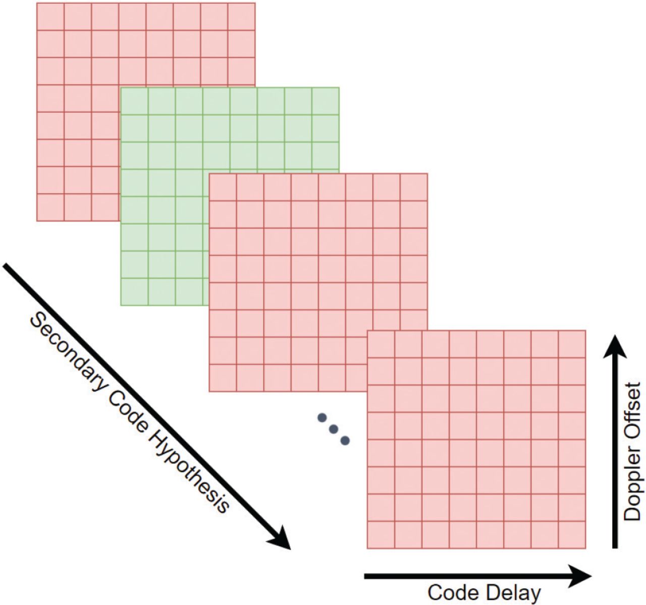
After computing the correlations for all the SCI hypotheses, the MH acquisition process generates CAF results with three dimensions representing code delay, Doppler shift, and the SCI value, respectively, as illustrated in Figure 3. It shows a multi-layer structure as the SCI values are discrete integer values. A search-and-detect procedure has to be conducted in order to find the best estimates of the parameters. Note that a CAF energy peak can be found within each layer, but only the ones that have the maximum energy (shown in green) among all layers lead to the final output acquisition results. In the present paper, we define a grid point in this 3D search space as a set of acquisition results.

• Download figure
• Open in new tab
• Download powerpoint

FIGURE 3

3D search space of MH acquisition for snapshot signals

2.3 Data Bit Ambiguity Issue

In order to achieve high-precision positioning with snapshot data, it is vital to obtain correct information about the SCI values of all satellites. The reason is two-fold:

1. To compute an accurate tiered code delay, which will leave a resolution of a full secondary code period for the navigation filter to determine the global time tag of the observables as described in Liu et al. (2021); only when accurate SCI values are known can the satellite transmission time be properly computed and the satellite coordinate errors can be within an acceptable range.

2. To ensure that the secondary code symbols are estimated correctly; it is necessary for the snapshot receiver to identify and correct the acquisition results when the hypothesis with opposite secondary codes are used. Only in this way will the carrier-phase measurements be free from half-cycle anomalies.

However, when applying MH acquisition for short snapshot signals, it is possible that the CAF energy could be exactly the same for a few sets of acquisition results. Although the code delay and Doppler offset measurements are identical among all sets of results, there is an ambiguity in the resulting SCI values. Such ambiguous outputs can occur in two scenarios:

1. There exist multiple SCI hypotheses that lead to exactly the same bits. This happens more often when the received signal is short and, thus, the N_S value is small.

2. There exist other SCI values that lead to secondary codes that are exactly opposite to the actual ones.

The second scenario results in an erroneous carrier-phase measurement candidate, which is half of a cycle off the actual carrier-phase measurement (Liu et al., 2021). These carrier-phase measurement anomalies, if not corrected, will result in failure of the IAR procedure in the navigation filter and denial of a high-precision positioning solution. These unwanted ambiguities in the SCI outputs refer to the DBA issue. Tackling this issue is the main target of this research.

As an example, Figure 4 shows all four possible ambiguous cases for the Galileo E1C pilot signal with a received signal length of 20 ms, for which six secondary code symbols are required to be computed by Equation (3). The green and pink rectangles represent the locations of the local replica secondary codes according to their SCI hypotheses. For each case, the rectangles are shaded with the same color (both green) if their secondary code symbols are exactly the same and different colors (green and pink) if they contain opposite bits. As can be seen in the first ambiguous case, SCI indexes of 5 and 6 lead to exactly the same secondary code symbols, both with the sequence of [1 1 1 1 1 1]; this corresponds to Ambiguous Scenario 1. For the other three cases, the pairs of ambiguous SCI values all lead to the exact opposite secondary code symbols and are, thus, shaded by different colors. For instance, Ambiguous Scenario 2 has an SCI of 2 and 24 that correspond to the sequences of [0 0 0 1 1 1] and [1 1 1 0 0 0], respectively. In these cases, the carrier-phase measurements suffer from half-cycle errors if the acquisition result sets with incorrect SCI values are chosen.

• Download figure
• Open in new tab
• Download powerpoint

FIGURE 4

SCI ambiguous cases for 20 ms of Galileo E1C signal

3.1 Overall Workflow

The purpose of the DBA Resolution (DBAR) is to ensure that valid measurements are provided to the SRTK engine. Before detailing the new proposed solution, it is important to, first, understand the typical workflow of the SRTK algorithm under nominal scenarios in which long integration times are used and no DBA issues are present. In these circumstances, as illustrated in Figure 5, the MH acquisition process generates only one set of results for each satellite. Then, together with the assistance data, the fractional code delay measurements are fed to a full period ambiguity resolution procedure in order to build the full pseudoranges. Note that, in some literature, this process is also referred to as integer millisecond ambiguities (van Diggelen, 2009). The method makes an estimate on the geometric range and flight time for each satellite based on the extensive use of assistance data, including the rough receiver coordinates, rough receiver time, and satellite ephemeris data that are used to compute the satellite positions. Based on these rough flight time values, an integer number can be computed for each satellite by integer rounding and, then, compensated for their factional code delays to form full pseudoranges. Note that van Diggelen (2009) has provided a conservative analysis on the acceptable assistance data error. He stated that, when the combined position and time error is less than 150 km, the millisecond integers can be found correctly. Finally, the resulting full pseudoranges and other measurements, including the SCIs, Doppler offsets, and carrier phases, are used in the SRTK engine to estimate high-precision PVT solutions. More specific procedures of the SRTK technique are described in Liu et al. (2021).

• Download figure
• Open in new tab
• Download powerpoint

FIGURE 5

The overall SRTK workflow for long snapshots that are free from DBA issues

However, when DBA issues arise, the workflow requires the inclusion of the DBAR process. As shown in Figure 6, the MH acquisition results now contain multiple ambiguous sets for each satellite. In the table, the superscripts of the measurements denote the satellite index and the subscripts from 1 to Mⁱ stand for the indexes of the acquisition result sets for satellite i, where Mⁱ is the total number of ambiguous sets of satellite i. Note that, for each satellite, the code delay measurements are identical for all the ambiguous sets, thus, the full period ambiguity resolution process is not impacted by the existence of ambiguous results. The only difference in this figure is that the transmission time differences among satellites are also computed in this process as they are critical input for the DBAR process. Ideally, the DBAR process would filter the acquisition results and generate a unique set of solutions for each satellite, just like in the previous nominal case. Then, filtered outputs are fed to the SRTK engine together with the full pseudoranges to obtain the PVT results.

• Download figure
• Open in new tab
• Download powerpoint

FIGURE 6

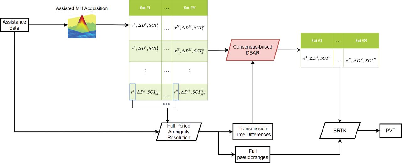
The overall SRTK workflow with the DBAR procedure for short snapshots

3.2 Satellite Independent Solution

As mentioned in Section 2.2, in order to find the unique SCI value that leads to the actual data bits encoded in the received signal, different SCI hypotheses should not lead to identical secondary code symbols or to those with exactly opposite signs. These conditions can be easily met if the received signal contains many symbols. However, when the snapshot recording is short and the N_S value is small, DBA issues start to arise. There is a limit to the duration of received signals until which we can still obtain a unique set of acquisition results instead of multiple ambiguous sets. For example, Figure 4 shows that, with a Galileo E1C signal duration of 20 ms, there are four ambiguous scenarios and a total of eight SCI values that could lead to DBA issues, which indicates that there is a 32% probability that this satellite cannot obtain a unique acquisition result set. We further expand this calculation and count the theoretical number of ambiguous SCIs (denoted by N_amb) for different lengths of signals. The results are presented in Table 2 together with other details such as N_S, the possibility of DBA to occur, and N_hyp, the maximum number of hypotheses for each ambiguous case (i.e., the maximum number of SCI candidates that lead to the same secondary code sequence).

It can be seen from Table 2 that, when applying the satellite independent solution, the DBA issue can be expected to be absent from the MH acquisition results of all satellites only when the collected Galileo E1C signal has a duration greater than 24 ms. Only under this condition can it be assured that the resulting snapshot carrier-phase measurements are free from half-cycle errors. In order to alleviate such limitations and ensure correct carrier-phase measurements for shorter integration times, an innovative method has been proposed and is described in the following section.

3.3 Consensus-Based Solution

The consensus-based solution is based on the fact that satellite transmission time differences can be obtained as a side product in the full period ambiguity resolution procedure described in van Diggelen (2009) and Yoo et al. (2020). Since we have a-priori knowledge about the whole secondary code sequence, the mapping from transmission times to the encoded secondary codes are already known, thus, the expected relationship between the SCI values of different satellites can be obtained as well. These relationships then work as a constraint for the SCI values obtained from the MH acquisition results.

The difference between the number of milliseconds that are compensated for by each satellite is equivalent to the flight time differences between satellites. The mentioned differences are also what really matters for the proposed method, since they can be directly converted into the integer millisecond parts of the transmission times between all satellites. The misalignment in flight times can be denoted as , where i stands for the satellite index. Note that a reference satellite needs to be chosen and this misalignment value is a relative quantity to the reference satellite. Another important point is that the reception time t_r is the same for all satellites. For this reason, we can build Equation (4): 4

where:

• C is a constant for all satellites. Since indicates a relative quantity to a reference satellite, this value also includes the receiver clock error that is common to all satellites.

• ΔTⁱ represents the other factors that may impact the total flight time of satellite i, such as satellite clock errors and atmospheric delays. These values can be computed based on assistance data as well.

• Rⁱ is an integer value that stands for the number of secondary code rollovers, since the transmission epochs of two satellites might be located at two different secondary code periods.

• T_SC = N_SC · T_S is the full secondary code period.

Equation (4) functions as the basis of the consensus-based solution; it sets a constraint for the SCI values since they have to be selected to ensure all the satellites fulfill this equation. The essential information we need to focus on is actually the consistency of the right side of the equation, which can be simplified to: 5

Note that the modulus operation is applied in order to avoid the inclusion of the unknown secondary code rollovers Rⁱ. This results in a real constant on the right side of the equation for all satellites, represented as C_frac, since it is a fractional value between 0 and T_SC.

The new method can be generally divided into six steps:

1. The MH acquisition generates all the SCI values that lead to a potential acquisition peak for each satellite, including those with correct secondary codes and those with exactly opposite signs. For each satellite, only one candidate is correct and results in the actual carrier-phase measurement; other candidates, however, could lead to half-cycle errors.

2. Compute the ΔTⁱ term for all the satellites based on the assistance data.

3. Solve the 1-ms Ambiguity Resolution for all satellites and then select a satellite as a reference to compute its flight time differences to all other satellites, which results in . Note that for the reference satellite is always 0.

4. Shift all potential SCI candidates (computed in Step 1) for each satellite by an amount corresponding to the flight time differences obtained in Step 3 and obtain the modulus of shifted indexes for each satellite.

5. Find a unique common integer value among the modulus of all shifted indexes (computed in Step 4). This process can be achieved by a weighted voting procedure, as described in Section 3.4. In this way, SCI ambiguities for each satellite are resolved.

6. Shift back the unique integer values obtained in Step 5 according to their flight time differences (by the same amount as in Step 4) and retrieve the actual SCI values for each satellite. Finally, filter out other measurement values that are corresponding to the wrong SCI candidates.

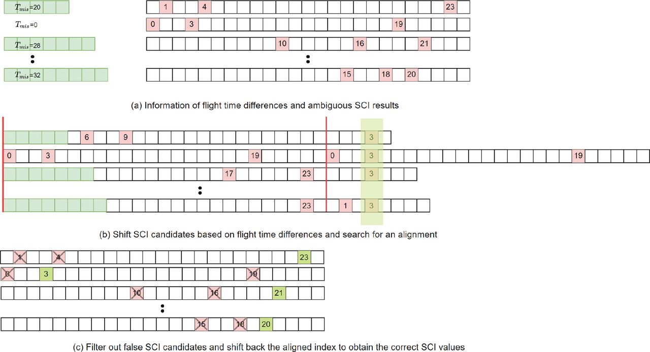
Figure 7(a) shows an example of MH acquisition results at the top-right corner; the red square boxes represent all the SCI hypotheses that lead to the CAF energy peak. Note that, in this example, the coherent integration time is 12 ms (thus, N_S = 4) and only Galileo E1C pilot signals are used. As it can be seen, each satellite has three ambiguous SCI candidates while only one of them is the correct one. The goal is to resolve this ambiguity and find the actual SCI value with the help of the flight time difference information , which is provided in the top-left corner. These differences are computed using the second satellite as reference.

• Download figure
• Open in new tab
• Download powerpoint

FIGURE 7

Example of DBA solution based on transmission time consensus

The next step is to shift all the SCI candidates for each satellite by an amount that corresponds to their flight time differences and update the SCI values, as shown in Figure 7(b). Note that the second satellite has been shifted by a full secondary code period in order to better illustrate the consistency among satellites under the secondary code rollover, which is taken into account by the modulus operation. Then, a common integer of 3 can be found based on the consensus among these shifted SCI values, while the other SCI candidate can be considered false and discarded. These false candidates are marked by a cross in the figure. Finally, by shifting back this common index with the same amount as , we can find the actual SCI values for each satellite. In this case, as shown at Figure 7(c), we can obtain [23, 3, 21, …, 20]. The carrier-phase measurements built based on these SCI values are then free from half-cycle errors.

3.4 Weighted Voting Based on Energy

In many actual recordings, the acquisition process can provide results that are prone to errors when the received signal strength is weak. When such errors exist in SCI results, it is possible that the proposed method cannot find a common shifted SCI value from all the satellites. In this case, the consensus is destroyed by a minority that shows an anomaly due to false acquisition. In order to still obtain a robust solution in these scenarios, it is proposed to assign each satellite with a different weight and perform a voting procedure to form the final consensus among all the satellites. A good metric for the voting weight is the energy magnitude obtained in the CAF. This addition brings two advantages:

1. The voting weight leverages the reliability of different satellites which results in a final solution that agrees more with the satellites with higher correlation peaks.

2. This step ensures that a unique solution can still be found even when a minority of satellites show anomalies and interrupt the procedure of finding the common index.

3.5 Practical Challenges of DBA

Even though the proposed method brings great benefits for signals with short coherent integration times, it is still not possible to totally solve all the DBA issues, especially when the number of acquired satellites is reduced. The effectiveness of this method depends on three factors:

• the diversity of the transmission times among satellites

• total number of satellites

• the number of ambiguous SCI hypotheses for each satellite, N_hyp

The first factor, the diversity of satellite transmission times, depends on the satellite-receiver geometry. It decides the flight times of each satellite and, since the reception time is common to all satellites, it results in the differences in the transmission times and SCI values among satellites. If all acquired satellites have very similar geometric distances to the receiver and result in almost the same flight times, the shifted SCI indexes as described in Step 4 of Section 3.3 would tend to be identical, and the procedure of maximum voting could fail to find a unique index at Step 5, remaining ambiguous.

The second factor, the total number of satellites, impacts the solution mainly because the more satellites that participate in the voting, the higher the chance that a unique solution can be obtained. The third factor, the number of ambiguous SCI hypotheses for each satellite, is decided by the number of secondary codes encoded in the snapshot signal N_S, which is higher for longer coherent integration times and lower for shorter signals. For these reasons, unsuccessful DBAR could still happen when the integration time is short and there is a limited number of satellites acquired. We performed experiments under these scenarios; the results are presented in Section 4.2.

4.1 Data Description

A total of 240 snapshot GNSS recordings were collected using a snapshot receiver designed by Albora Technologies. The receiver was connected to a high-end antenna (Septentrio PolaNt-x MF) that was located in an open-sky environment in Barcelona, Spain. Each snapshot had a total duration of 200 ms, however, they were truncated into snapshots with different durations in order to test the performance of the proposed method with shorter lengths of signals. The sampling rate of the collected snapshots was set at 31.8 MHz.

4.2 Experimental Setup

Since the traditional satellite independent method can already solve DBA issues when the snapshot length is longer than 24 ms, the experiments in the present work were focused on snapshot lengths of {4, 8, 12, 16, 20} ms. The acquisition module was running in full coherent integration mode using the whole length of the truncated snapshot data. In order to get the true values of the SCI for each satellite, the data set was processed in advance with a long integration time of 40 ms using the satellite independent method to ensure that the detected SCI values were reliable. The results of the new method were then compared to the corresponding true values in order to evaluate its performance variation under different snapshot durations.

In these experiments, only the Galileo E1C signal was analyzed. This is because only L1-band signals were collected and other pilot signals in this band had longer secondary code durations. For example, for BDS B1C signals, one secondary code symbol lasted 10 ms when the full sequence contained 18,000 bits that lasted 18 seconds, as shown in Table 1. Since our targeted snapshot duration was generally under 20 ms, the resulting number of symbols N_S for these signals was basically less than 2, which does not bring much benefit to the DBAR process. For this reason, we decided to focus on Galileo E1C signals.

4.3 Experimental Results

There are two metrics that shold be taken into account when evaluating the performance of the consensus-based method:

• Percentage of Uniqueness P_u: This value represents the success rate of achieving the DBA Resolution. It shows the percentage of snapshots that a unique set of acquisition result can be found, as described in Step 5 of Section 3.3.

• Percentage of Correctness P_c: The correctness of the final filtered acquisition results; for this, we need to test if the resulting unique set of SCI values for all satellites are the same as the true values. A simple way to evaluate this is by verifying the correctness of the shifted index value, which is computed in Step 4 of Section 3.3. In this way, we only need to make the comparison once, instead of comparing SCI values for each satellite.

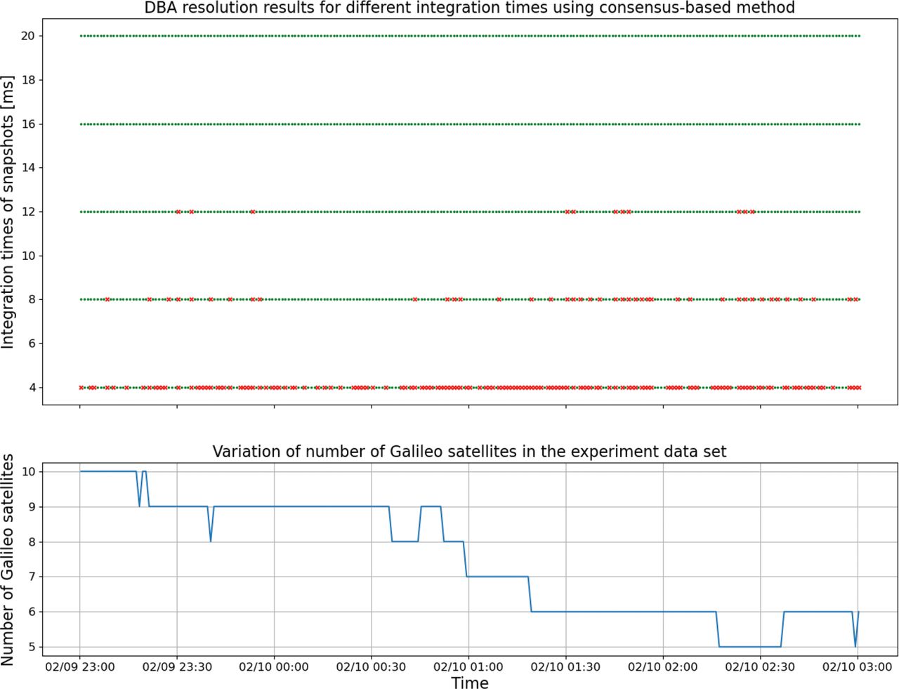
The snapshot processing results are shown in the upper panel of Figure 8, where green dots represent results with DBA issues that have been successfully resolved and result in a single set of acquisition outputs, while results of red crosses show that the SCI ambiguities remain after the filtering process. The lower panel of Figure 8 shows the number of Galileo satellites that were acquired successfully. To evaluate the performance in terms of uniqueness for the consensus-based method, we computed P_u for different integration times; their values are listed in Table 3.

• Download figure
• Open in new tab
• Download powerpoint

FIGURE 8

DBA Resolution results after applying the consensus-based method for different integration times

Contrary to the percentage of uniqueness is the probability of DBA, which is also represented by the orange line (with triangle markers) in Figure 9. We can see that, by applying the proposed method, a unique solution can be obtained for all snapshots longer than 12 ms. As a comparison, the traditional satellite independent method (denoted by the blue line with cross markers) needs at least 24 ms of snapshot length to achieve this. When the snapshot length goes even shorter, the new method still shows superiority as it results in a much lower possibility of DBA.

• Download figure
• Open in new tab
• Download powerpoint

FIGURE 9

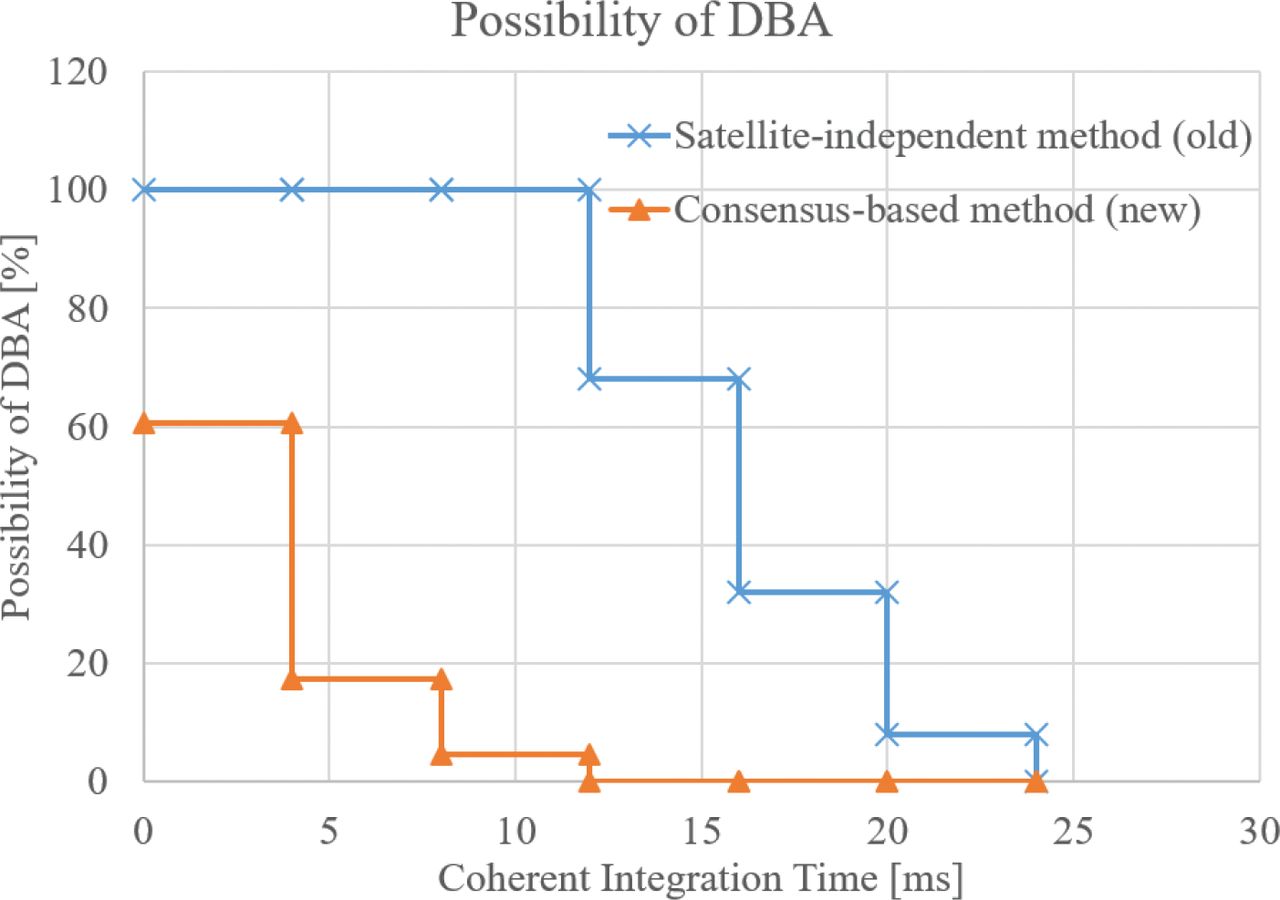
Probability of DBA issues to occur for Galileo E1C signal using the traditional and proposed methods

As for performance in terms of the correctness, the P_c values are computed and listed in Table 3. As it can be seen, basically all the actual SCI values were filtered out correctly as long as a unique SCI set could be found. The only exception is when the snapshot is less than 4 ms. A few snapshots have been fixed to the wrong SCI values, which might be caused by false acquisitions due to the short integration time and because only two secondary code symbols were involved. The larger the number of N_hyp, the more difficult it is for DBA to be solved correctly.