

Article Figures & Data
Figures
- FIGURE 1
NLOS and multipath effects in GNSS satellites lead to high localization uncertainty in urban areas, especially along the cross-street direction. The pink ellipse depicts uncertainty in the receiver position estimate. This figure is adapted from Wang et al. (2013b)
- FIGURE 2
Our proposed technique on set-valued shadow matching using zonotopes to leverage constrained zonotopes and efficiently represent buildings, shadows, and a set-valued receiver position estimate; note that the 2D group plane is shown as having volume only for illustration’s sake.
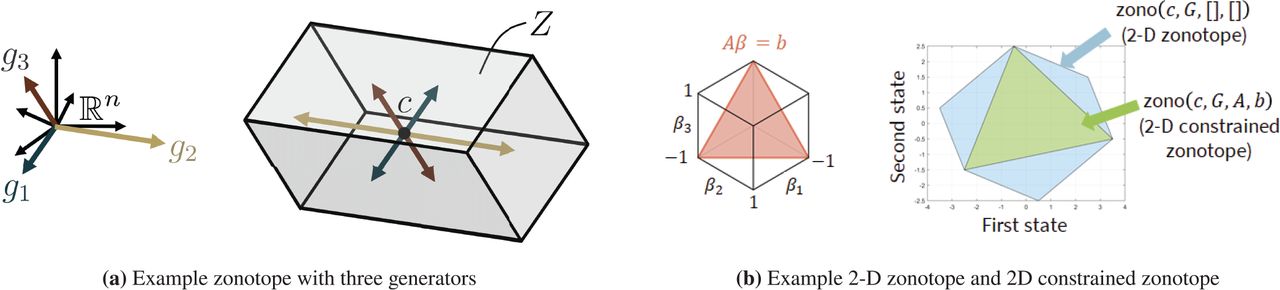
- FIGURE 3
Subfigure (a) is a zonotope (grey volume) with no constraints and three generators; subfigure (b) shows a 2D zonotope (blue) and a constrained zonotope (green) with constraints shown in red on the left.
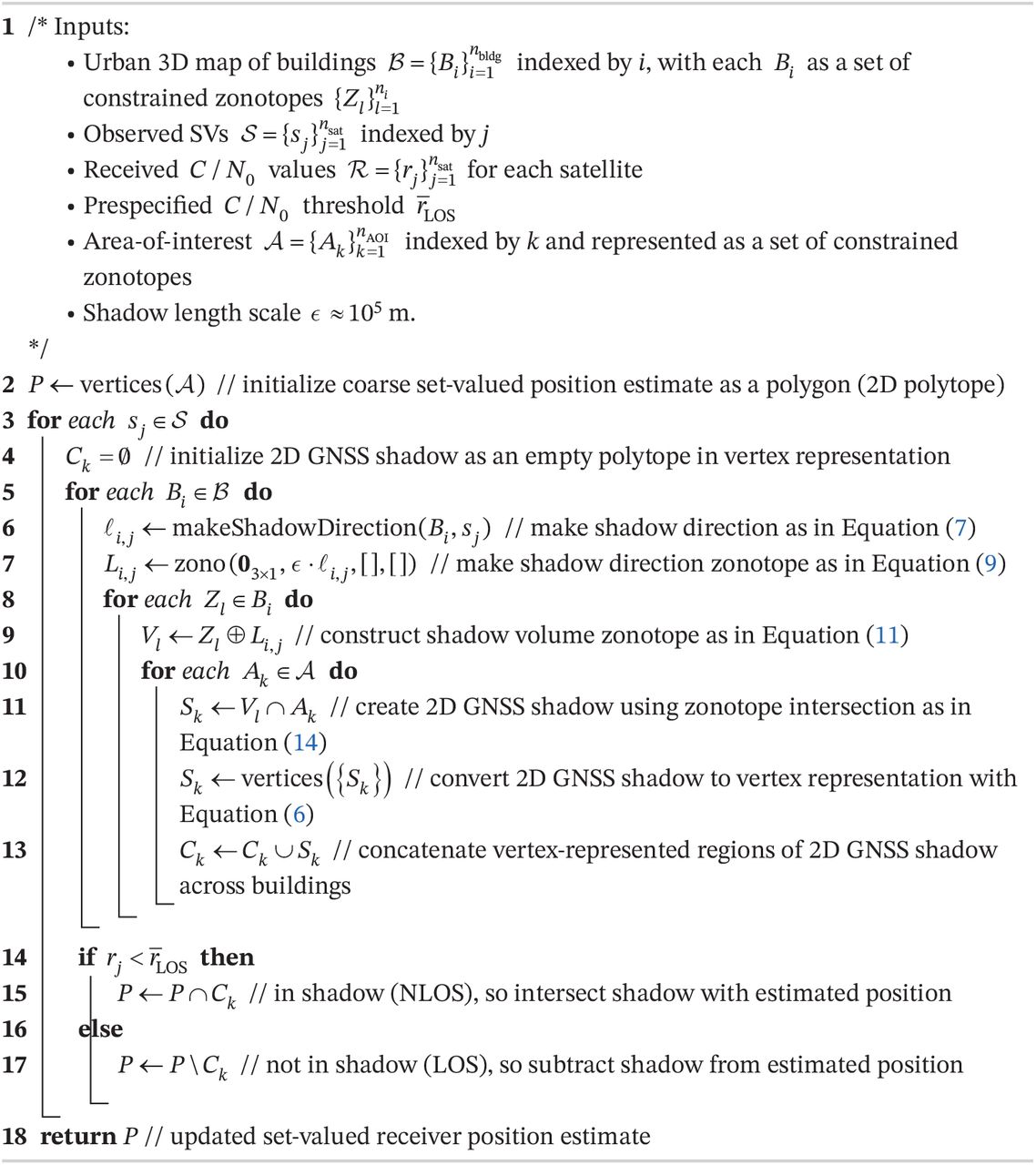
- ALGORITHM 1
 // zonotope shadow matching (Snapshot)
 - FIGURE 4
Constrained zonotopes improve Minkowski sum computation time by an order of magnitude over a standard vertex representation (each red plus denotes an outlier).
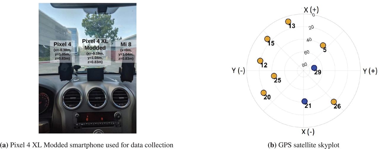
- FIGURE 5
Subfigure (a) is the experiment test platform utilized to validate the proposed ZSM via publicly-available Google Android data sets in Fu et al. (2020). Subfigure (b) shows the skyplot for a particular receiver location with nine visible GPS satellites. The GPS satellites are represented by circles with LOS satellites in blue and NLOS (simulated effects) in dark yellow.
- FIGURE 6
Subfigure (a) is an illustration of the experiment setup, while subfigures (b)-(f) represent iterations of the proposed ZSM algorithm. The magenta area is the receiver position estimate and the blue areas are shadows.
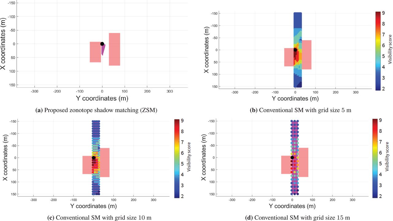
- FIGURE 7
The ZSM position estimate in subfigure (a) has a comparable estimation error to the conventional SM results in subfigures (b)-(d). Note that the ZSM error does not depend on a predefined grid density.
- FIGURE 8
Our GPS software simulation pipeline uses two publicly-available software: GPS-SDR-SIM (Ebinuma, 2018) and SoftGNSS (Rojas, 2011). For a given true receiver location, we simulated the C/N0 values and, thereafter, induced NLOS effects using a 3D building map of San Francisco.
- FIGURE 9
Preprocessing 3D building map of San Francisco: (a) shows the vertex representation, wherein the vertices of each building are separately color-coded; and (b) represents each building as a constrained zonotope, which is given as input to our proposed ZSM algorithm.
- FIGURE 10
Our second simulation experiment using a 3D map of San Francisco: Subfigures (a) and (b) show the initial AOI and surrounding buildings, while (c) shows the skyplot for the true receiver position with LOS satellites in blue and simulated NLOS in dark yellow.
- FIGURE 11
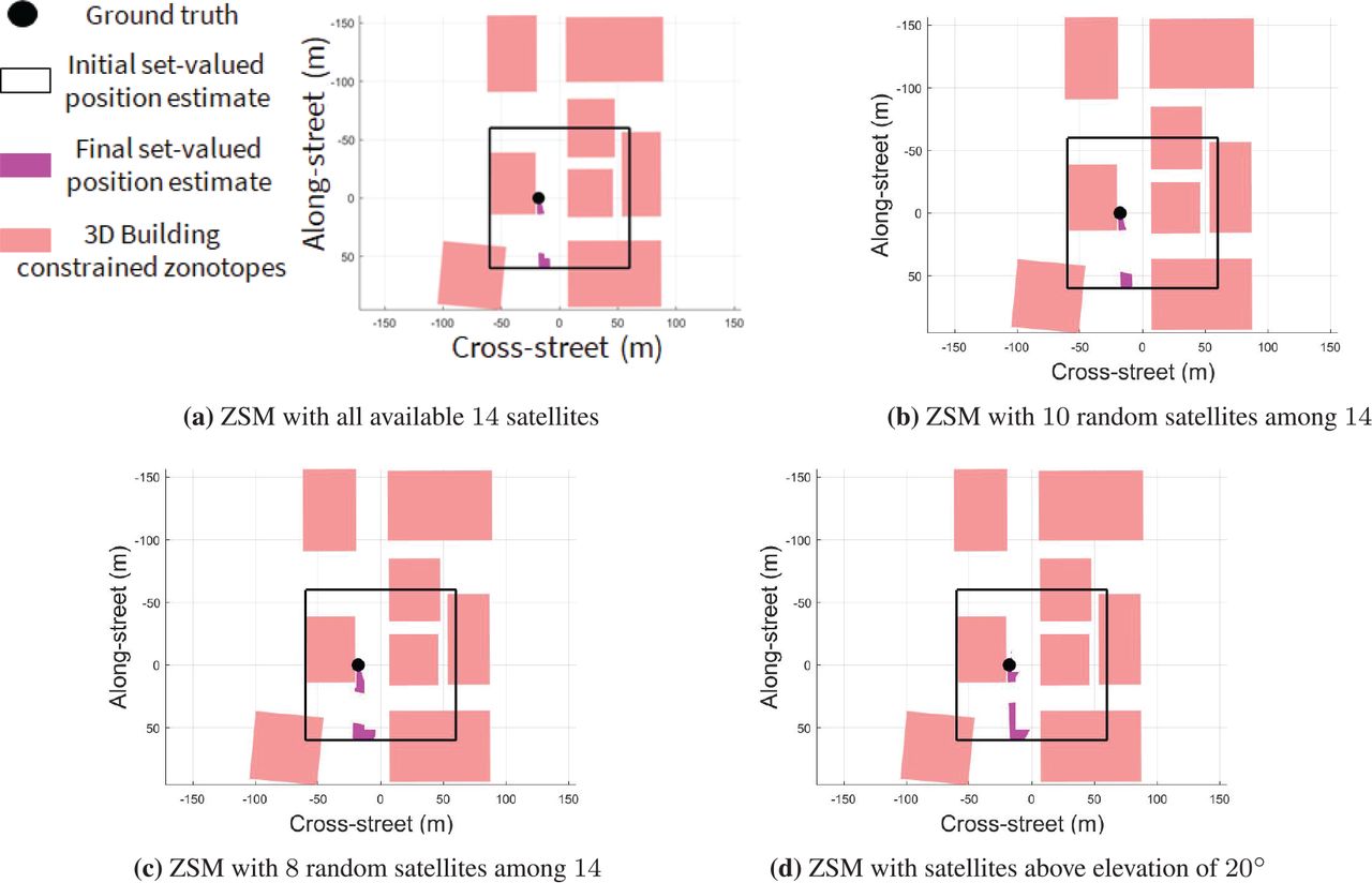
Our proposed ZSM algorithm estimates the receiver position with high precision (i.e., the area of the receiver estimate set is small), but produces a bimodal output in this example. The mode containing the true receiver position is not majorly affected by the consideration of different subsets of the available GPS satellites.
- FIGURE 12
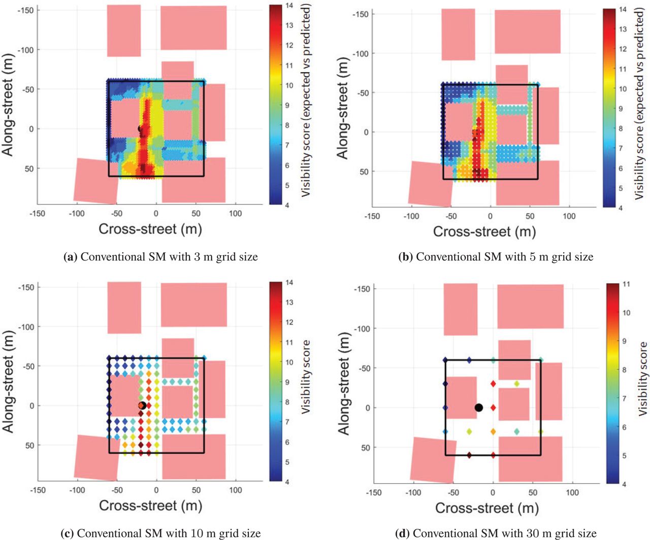
The results of conventional SM strongly depend upon grid size (a denser grid is more accurate). However, in this case, the uncertainty bounds in the conventional SM are over 100 m, indicating that ZSM is much more precise.
- FIGURE 13
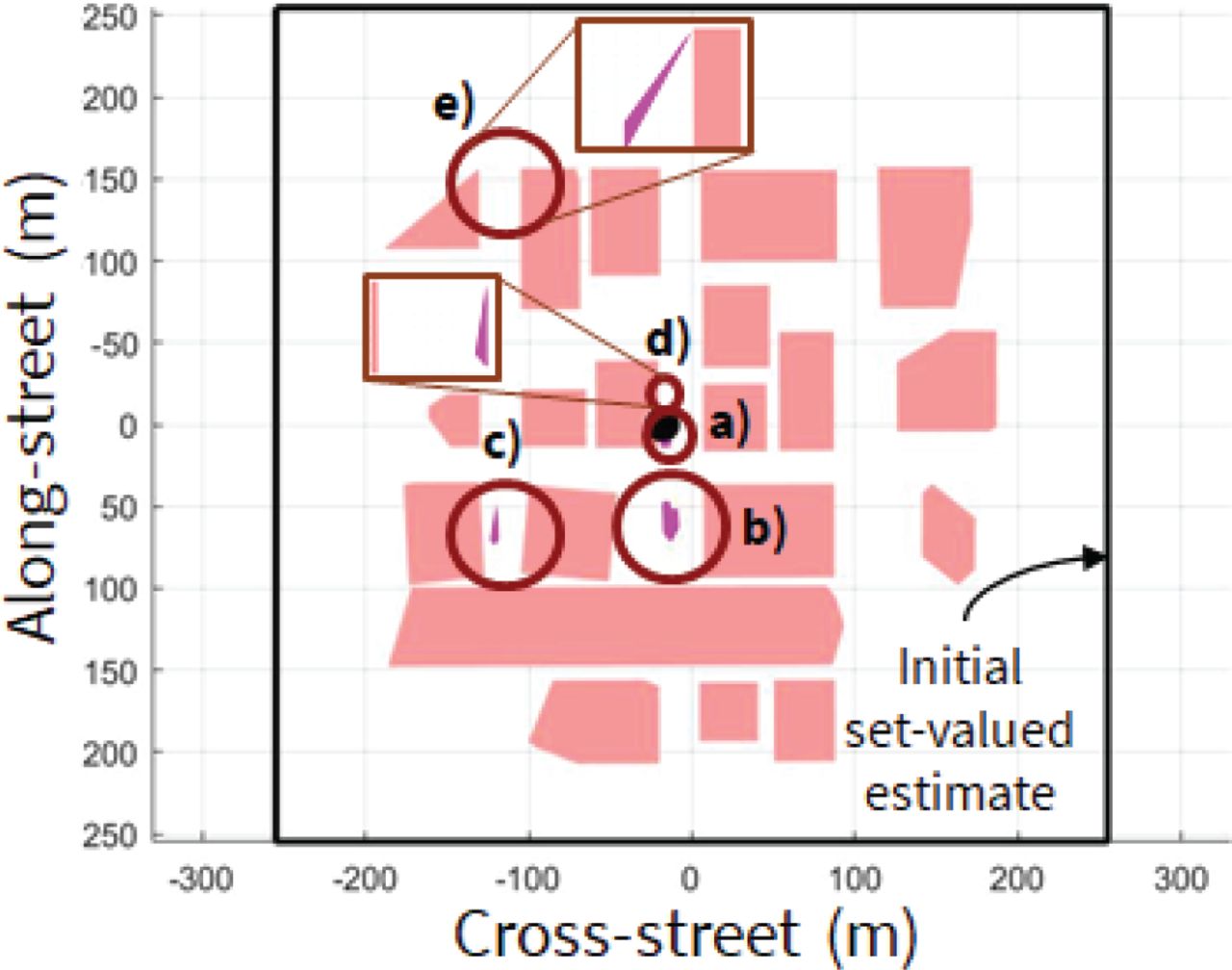
ZSM produces a set-valued estimate with many disjoint components (magenta) when considering many buildings (pink) and a large AOI. However, each disjoint component is small, so fusing a ZSM estimate with other estimates to eliminate multi-modality can produce an accurate receiver position estimate.
- FIGURE 14
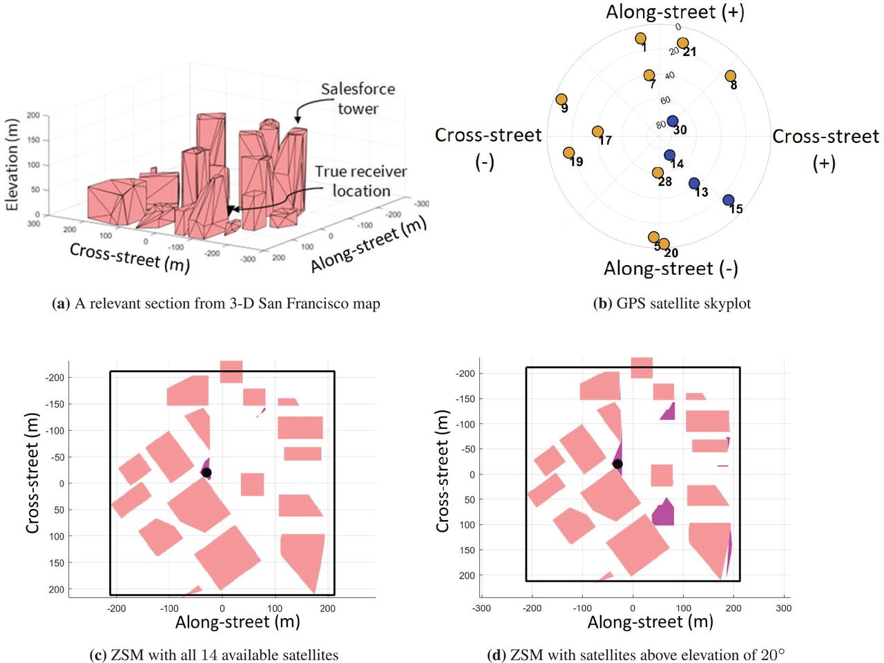
Our third simulation experiment in a different location using the 3D map of San Francisco; (a) shows a relevant section of 3D map near the Salesforce tower wherein the distinction between cross-street and along-street is not well-defined; (b) shows the skyplot with respect to the true receiver location with 14 visible GPS satellite, the GPS satellites are represented by circles with LOS satellites in blue and NLOS [simulated effects] in dark yellow; (c) shows the final set-valued estimate of the receiver position estimated by our ZSM when all 14 satellites are considered; and (d) shows this set-valued estimate using satellites with elevation > 20°. We demonstrate that in both cases, our ZSM successfully detects the mode containing the true receiver location, while exhibiting a higher centroid error and bounds for the reduced six satellite case as compared to the full 14 satellite case.


Tables
- TABLE 1
Performance Comparison Results for ZSM vs Conventional SM on a Simulation Experiment With two Buildings Seen in Figure 6(a) and Nine GPS Satellites seen in Figure 5(b).
Algorithm Error w.r.t true location (m) [Cross-street, Along-street] Bound (m) [Cross-street, Along-street] Avg. computation load across 100 runs (s) Offline Online Proposed ZSM [3.46, 16.05] [17.87, 50.11] 1.7e-4 0.39 Conventional SM with grid sizes 5 m [3.00, 5.00] [59.58, 447.48] 1524.41 1.66 [2.00, 0.00] [3.00, 0.00] 10 m [3.00, 0.00] [66.72, 455.82] 405.33 0.08 [7.00, 0.00] [3.00, 10.00] 15 m [3.00, 0.00] [73.54, 463.10] 296.32 0.04 [3.00, 15.00] [3.00, 30.00] - TABLE 2
Performance Comparison Between ZSM and Conventional SM Based on a 3D Map of San Francisco
Algorithm Centroid error w.r.t true location (m) [Cross-street, Along-street] Bounds (m) [Cross-street, Along-street] Average computation load across 100 runs (s) Offline Online Proposed ZSM 14 satellites [1.2, 8.1] [5.8, 16.2] 162.5 4.4 [4.6, 58.8] [9.8, 24.5] 10 random satellites [0.9, 6.8] [6.1, 16.4] 162.5 4.2 [4.8, 53.8] [9.7, 13.1] 8 random satellites [1.4, 13.1] [18.3, 26.8] 162.5 3.0 [3.5, 54.3] [7.6, 24.8] Satellites with elevation > 20° [1.7, 10.2] [0.5, 3.3] 162.5 2.4 [1.9, 7.0] [8.7, 20.2] [4.9, 48.5] [16.8, 29.9] Conventional SM (all available 14 satellites) 3 m [0.0, 3.0], [0.0, 6.0], [0.0, 9.0] [173.2, 214.5] 91204.0 2.8 [0.0, 12.0], [3.0, 12.0], [0.0, 48.0] [3.0, 48.0], [0.0, 51.0], [3.0, 51.0] [0.0, 54.0], [3.0, 54.0], [3.0, 57.0] 5 m [2.0,10.0] [173.1, 215.6] 34389.9 1.2 [2.0, 50.0], [3.0, 50.0], [3.0, 55.0] 10 m [2.0, 10.0] [192.1, 221.6] 6874.1 0.3 [2.0, 50.0] 30 m [12.0, 60.0] [224.5, 261.8] 1433.4 0.1 Note: For proposed ZSM, we performed comparison analysis across different GPS satellite subsets, while for conventional SM we compared the performance for different grid resolutions. The 14 satellites can be seen in Figure 10(c)
No. of buildings Centroid Error @ Bound (m) [Cross-street, Along-street] Avg. computation load for 100 runs (s) Offline Online 8 a) [1.2, 8.1] @ [5.8, 16.2] 162.5 4.6 b) [4.6, 58.8] @ [9.8, 24.5] 14 a)[1.2, 8.1] @ [5.8, 16.2] 165.4 9.4 b)[4.6, 58.8] @ [9.8, 24.5] c) [102.4, 63.9] @ [4.9, 25.2] 20 a) [1.2, 8.1] @ [5.8, 16.2] 169.8 12.2 b)[4.6, 58.8] @ [9.8, 24.5] c) [102.4, 63.9] @ [4.9, 25.2] d) [1.7, 10.1] @ [0.4, 3.3] e) [87.0, 155.9] @ [0.3, 0.5]


Jump to section
Related Articles
Cited By...
- No citing articles found.