

Abstract
One of the fundamental problems of robotics and navigation is the estimation of the relative pose of an external object with respect to the observer. A common method for computing the relative pose is the iterative closest point (ICP) algorithm, where a reference point cloud of a known object is registered against a sensed point cloud to determine relative pose. To use this computed pose information in downstream processing algorithms, it is necessary to estimate the uncertainty of the ICP output, typically represented as a covariance matrix. In this paper, a novel method for estimating uncertainty from sensed data is introduced.
1 INTRODUCTION
One of the key algorithms used when working with 3D point clouds is the iterative closest point (ICP) algorithm introduced by Chen and Medioni (1992) and Besl and McKay (1992). Since then, the ICP algorithm has been used in many robotics applications such as search and rescue, powerplant inspection, shoreline monitoring, and autonomous driving (Pomerleau et al., 2015). It is also used in 2D or 3D self-localization methods such as simultaneous localization and mapping (SLAM; Mendes et al., 2016). Input data for the ICP algorithm can come from lidar, monocular, or stereo vision sensors.
The ICP algorithm consists of iterating through the following two steps:
For every point in the measured point cloud, find the closest point in the reference point cloud.
Compute the best 6D pose (location and orientation) to align each measured point with its closest reference point. Note that finding the best 6D pose to align points with a 1-to-1 correspondence can be solved in closed form using quaternions or the singular value decomposition (SVD) of a 3×3 matrix (e.g., Arun et al. [1987], Horn [1987], and Horn et al. [1988]).
By iteratively executing this process, the ICP algorithm outputs the best-fit 6d pose, as well as the correspondence between the sensed and reference points. This best-fit rotation and translation estimate is what can be used by downstream algorithms to complete their tasks.
To use a position and rotation estimate in a navigation framework, knowing the accuracy of the derived estimate can be as important as the estimate itself. For example, many robotics applications use the output of ICP to form a pose graph, where the 6d transform between two point clouds is used to estimate the movement of the robot. To estimate the robot trajectory over time, a trajectory that is the best match (probabilistically) to the measured 6d transforms is found. What makes the best match depends on the uncertainty estimated for the ICP output. Unfortunately, as mentioned in Censi et al. (2008), most ICP algorithms do not return estimates of their own uncertainty. Therefore, in this paper, we look to improve the estimation of the uncertainty obtained when running the ICP algorithm. We do not propose modifying the ICP algorithm, itself, but simply the estimation of its uncertainty after ICP has converged to a solution. Therefore, Section 1.2 only covers methods for estimating uncertainty, and not the ICP algorithm itself.1
The motivating application for this paper is two aircraft attempting to fly in formation. There will be some safety margin built into the desired (relative) location of the aicraft to ensure a collision does not occur. However, if the ICP uncertainty is high, then the safety margin can be violated even without external disturbances due to errors in the ICP algorithm. This, combined with external disturbances, can quickly lead to catastrophic failures. Therefore, modeling the safety margin using an accurately estimated uncertainty is vital to ensuring safe operation. The focus of this paper is computing an accurate estimate of the uncertainty of the ICP output pose.
1.1 Notation
For clarity, we utilize the following notation in this paper:
Scalar: denoted by a non-boldface letter (e.g., k or N)
Vector: denoted by a boldface lowercase letter (e.g., n)
Matrix: denoted by a boldface uppercase letter (e.g., K)
Set: denoted by curly brackets (e.g., a set of vectors {pr}); the elements of the set are denoted as pr,i, where i is the index of that element.
Identity matrix: denoted by I followed by a subscript denoting its size (e.g., I6 is a 6 × 6 identity matrix)
1.2 Prior Work
To understand how uncertainty has been computed in the past, it is necessary to precisely define the objective of Step 2 in the ICP algorithm. The second step of the ICP algorithm is based on finding the relative pose that minimizes the sum of squared distances between the reference points and the sensed points. This step optimizes the following cost function (Markley & Mortari, 2000):
 1
1
where R and t are the relative rotation and translation between the reference and sensed points, ps,i is the i-th sensed point, ϕ(·) is a function that takes in an index to a point in the sensed cloud and returns an index to a matching (closest) point in the reference cloud, and pr,ϕ(i) is the position of the ϕ(i)-th point in the reference cloud.
As the solution to Step 2 is a least-squared problem, there are well-known methods for computing the covariance for the result. We term this the Jacobian method and describe it in the next section. We then describe some modifications that have been made in the literature to obtain more accurate uncertainty estimates. In simulation, the true covariance of this result can be obtained through a Monte-Carlo method.
1.2.1 Jacobian Method
The second step of the ICP algorithm is based on finding the relative pose that minimizes the sum of squared distances between the reference points and the sensed points defined in Equation (1). To understand the uncertainty resulting from this step, we will represent this step as a least-squares equation using normal form, yielding:
 2
2
where zi=ps,i – Rpr,ϕ(i) – t is a 3-vector and consists of an x, y, and z element, and x is a vector of changes to the relative pose expressed as:
 3
3
where tj is the j-th element of the three-element translation vector, rj is the rotation around the j-th axis, and J is the differential change in z with respect to tj and rj Specifically:
 4
4
The weighted least-squares problem solution can be solved as:
 5
5
where W is the weighting matrix. For data with a known covariance, cov(z), W = cov(z)−1, which also means W is symmetric. To find the covariance of x:
 6
6
 7
7
 8
8
 9
9
 10
10
Note that, when computing the covariance using the Jacobian method, we are assuming that the first step of the ICP algorithm perfectly matches every sensed point to the correct point in the reference model. With real data, however, there are two sources of error that are not considered by the Jacobian method. First, because the reference model consists of a set of points, there may not be a point at the exact location that the sensed point represents. Second, even if there was a reference point at the exact noise-free source of the sensed point, Step 1 of the ICP algorithm may match the sensed point to the wrong reference point. If we were to think of the reference model as a set of points lying on a surface, both of these noise sources introduced lose information along the surface, but preserve information orthogonal to the surface.
1.2.2 Advanced Methods
In Brossard et al. (2020), Censi (2007), Landry et al. (2019), Mendes et al. (2016), and Prakhya et al. (2015), more advanced methods of estimating ICP covariance are introduced. Censi (2007) lays the groundwork for this area of research by introducing a closed form estimation of ICP’s covariance that considers the additional error sources described above and demonstrates it on a 2D scan matching problem. Prakhya et al. (2015) extends Censi’s method into a 3D application. Mendes et al. (2016) utilizes this technique to apply ICP to a ground robot SLAM application. Brossard et al. (2020) examines the sources of error named by Censi: wrong convergence, underconstrained situations, and sensor noise. The most comparable work to ours was found in Prakhya et al. (2015). We describe how this method (termed the Prakhya method after the first author) solves for ICP covariance in the following subsection.
Prakhya et al. (2015) implements a closed form method of estimating the uncertainty of an ICP fit. The key insight of this method is finding a method to include the ICP cost function (Step 1 of ICP) within the Jacobian computation. The output covariance is calculated through Equations (11) and (12):
 11
11
 12
12
where x is the output state vector, cov(x) is the covariance of the output pose, C is the cost function optimized by ICP, and z is the input point vector.
Derivation: Let F be the ICP function where x = F(z). The first-order Taylor series approximation at z = z0 is then defined as:
 13
13
 14
14
To take the covariance of this form, the constants F(z0) and  can be ignored. Substituting into the expression, cov(Bz + c) = Bcov(z)BT, the covariance can now be defined as:
 15
15
F, however, is not in closed form and it is difficult to compute the partial derivative of F with respect to z0. Censi (2007) solves this problem with the implicit function theorem:
 16
16
Thus, substituting Equation (16) into Equation (15) yields the solution in Equation (12).
While this approach leads to significantly more accurate uncertainty results, the work introduced in this paper has two significant advantages over prior work. First, prior work has assumed the input covariance from the sensors is known a priori. This requires careful characterization of the sensors and may be violated as temperature or other environmental conditions change. We remove the requirement of a priori characterization in this work. Second, the approach proposed in this paper is computationally much faster than the Prakhya approach. Furthermore, we believe it to be conceptually easier to understand, enabling greater understanding of the uncertainty estimation problem for the ICP algorithm.
Another work that bears some similarity to our approach is Guehring (2001). In this work, Guehring propose modifying (weighting) the ICP least-squares solution by what we call the point-to-point method in this paper. Unfortunately, it does not show how this weighting can be used to compute an uncertainty (covariance) estimate for the final ICP results, nor does it show how this weighting affects the covariance estimate. Therefore, we do not directly compare against this approach in our results section.
1.3 Motivation/Test Scenario
This research is motivated by the problem of automated aerial refueling (AAR). Aerial refueling is the process of transferring fuel from one aircraft (the tanker) to the receiving aircraft while in flight and is a key enabler of Air Forces around the world. Currently, a human is used to guide the boom (a large pipe that protrudes from the back of the tanker) into the correct spot on the receiving aircraft. AAR proposes to automate the task of guiding the boom and requires a very accurate relative pose between the tanker and receiving aircraft. To accurately estimate relative pose, our research group has proposed using stereo computer vision in Anderson et al. (2021), where two cameras are mounted to the underside of the tanker aircraft. Stereo block matching is applied to the two images from the cameras to generate a point cloud representing the object in the visual field. Then, the ICP algorithm is used to fit a known model of the aircraft against the visually generated point cloud to estimate the output pose. This process is outlined in Figure 1. Noise may be introduced at multiple levels throughout this process; there may be pixel error in the cameras or the wrong features may be matched in stereo block matching, for example. To guarantee safe operation of the AAR application, the uncertainty in the system must be carefully evaluated and characterized. The covariance estimation methods proposed in this paper were tested on a complete simulation environment of the AAR application, enabling us to identify and evaluate the uncertainty due to different sources of error in the pipeline.
Stereo vision pipeline for automated aerial refueling (AAR)
In the remainder of this paper, we introduce our new technique for estimating covariance information of the ICP algorithm in Section 2. We present some preliminary results of our technique in Section 3, and conclude the paper in Section 4.
2 METHODOLOGY
To enable accurate estimation of the ICP uncertainty while considering the point matching (first) step of the ICP algorithm, we propose a Kalman filter update-based technique. In this section, we first introduce the Kalman filter-based approach, while subsections fill in details necessary for the implementation of this approach.
There are three key attributes of the Kalman filter that we use to properly estimate the covariance of the ICP algorithm, namely:
The Kalman filter is a least-squared estimator. Typically, the Kalman filter is used to perform a least-squares estimate using both dynamics and measurement updates. In this case, however, we will be doing just a multi-measurement update step (i.e., no dynamics for this system). This attribute shows that a Kalman filter can be used to properly estimate the covariance of a least-squares solution.
As shown in Sorenson (1966), as long as the measurements are not correlated, different measurements from the same time step can be applied in any order to the Kalman filter and the same result will be achieved. This enables us to create a computationally efficient algorithm that applies the measurement from only one point match at a time. Even though only the current estimate and covariance are stored, the final covariance will accurately reflect the impact of all point matches in the ICP algorithm.
The H or measurement matrix of the Kalman filter can be used to express in which direction a particular measurement has information. By properly choosing the H matrix, we can create a covariance matrix that is an accurate representation of the ICP uncertainty. This concept of a measurement’s direction is key to properly estimating the uncertainty of the ICP algorithm and will be discussed in detail later in this section.
Having motivated our choice of a Kalman filter, we show our specific implementation for this problem in Algorithm 1. Note that this algorithm is implemented after the ICP algorithm has completed execution, meaning we have both the best relative pose estimate (R, t) between the point clouds and a mapping, ϕ(i), that relates points in the sensed cloud to points in the reference cloud. Also note that the  values are incremental rotations around the 1st, 2nd, and 3rd axes.

Kalman Filter-Based ICP Covariance Estimation
In Algorithm 1, we start with a large initial value for the covariance (theoretically, infinity) and, with each measurement reduce the uncertainty depending on the new information given by the measurement. The unique aspects of our approach include:
The measurement covariance is estimated from the data rather than being an input. The actual calculation is shown on Line 4 in Algorithm 1 and is further discussed in Section 2.1.
Each measurement only reduces the covariance in a particular direction determined by H. The key working principle is that the measurement model, H, is constructed so that each sensed point only provides information (a reduction in covariance) in the direction denoted by the vector, n. The underlying assumption is that if there were any error orthogonal to the normal vector, that error would cause the sensed point to be registered to the next point over. Thus, all the information orthogonal to the normal vector is hidden from the ICP algorithm while the information parallel to the normal is preserved. Sections 2.2 and 2.3 describe two approaches to computing the normal vector, n.
2.1 Measurement Noise Estimation
Any approach to calculate the output noise must have a good understanding of the input noise. Note that the papers cited in Section 1.2.2 assumed that the input noise was known a priori. In our application, however, we are generating point clouds from a stereo vision setup. An inherent property of point clouds generated from stereo cameras is that the noise is strongly and non-linearly dependent on range. Thus, it is necessary to re-compute the input noise of the sensor for each image pair.
In a previous automated aerial refueling paper by Johnson et al. (2017), this error was characterized every 0.5 m from 30- to 100-m away from the camera. To utilize this method, however, creates a heavy characterization requirement. Nor can it take into account in-flight scenarios such as rain or out-of-focus cameras that may cause a change in the input uncertainty.
Therefore, instead of attempting to pre-characterize the sensor noise, we propose estimating the input noise from the data itself. Specifically, we can estimate the measurement noise,  , as the mean squared error of the distances between the matched points as shown on Line 4 of Algorithm 1. Assuming the ICP algorithm has converged onto the correct global minimum,
  should accurately reflect the variance of the sensor noise orthogonal to the local surface.
Note that, for this calculation to be valid, there are a few assumptions that should be satisfied. First, the ICP algorithm needs to converge to the right solution. Similar to the other advanced approaches described in Section 1.2.2, the proposed algorithm does not account for the possibility of the ICP algorithm converging to an incorrect solution. Second, we assume that the sensor noise is evenly distributed in all directions, following a spherical Gaussian distribution that is identical for each sensed point. Third, we assume all the sensed points are independent of each other. In Section 3, we present results demonstrating the efficacy of the proposed approach and its robustness to different imaging conditions.
2.2 Computing n from Point-to-Point Constraints
To execute the Kalman filter-based covariance estimation approach outlined in Algorithm 1, the ComputeNormal function must be defined. In this subsection, we describe a simple approach—the point-to-point method—to estimating the normal that leads to improved covariance results compared with the Jacobian method.
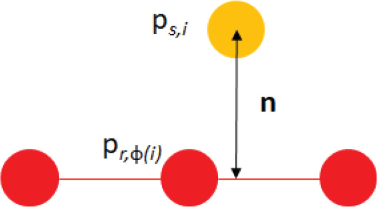
The point-to-point method, illustrated in Figure 2, computes the normal vector as the difference between the sensed point (i) and its corresponding reference point (ϕ(i)). Because this vector should be normalized, it is computed as:
 17
17

An example n vector from the point-to-point method
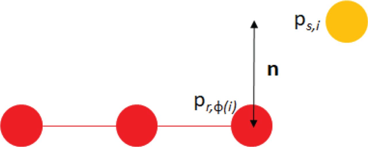
While this method works well in general, we also found that when the noise is small and/or the reference points are spread far apart, the normal vectors generated by this method can be significantly different than the true normal vectors of the surface defined by the set of reference points. For example, consider the example shown in Figure 3. The true normal of the reference surface should be pointed straight up as the reference points are in a horizontal line. Due to the small error in the true normal direction compared with the spacing between the reference points, however, the computed normal in this case will be significantly different from the true normal.

An example point-to-point scenario that generates a normal vector with significant error
To overcome this weakness of the point-to-point approach, we introduce another approach for estimating normal vectors—point-to-plane—in the following subsection.
2.3 Point-to-Plane Approach for n Estimation
The basic idea behind the point-to-plane approach is illustrated in Figure 4. The reference surface is locally approximated by forming planes between reference points that are close together. Then, rather than simply computing the unit vector to the closest reference point, the normal is computed to the closest plane. Note that there are several variants of the ICP algorithm that utilize a point-to-plane technique to try and improve the robustness of the ICP algorithm itself, e.g., Low (2004) and Segal et al. (2009).

A simplified illustration of the point-to-plane approach for computing n
In this application, n was found using a brute-force method. From the reference point cloud, the set {c} is populated from the eight closest neighbors in the reference model to Pr,ϕ(i). For each combination of two points in set {c}, a plane is defined between Pr,ϕ(i) and the two points, leading to different candidate planes. This produces a set of unit normal vectors local to Pr,ϕ(i). The plane normal vector with the greatest absolute dot product against the point-to-point normal vector is selected as the new n value.
While the point-to-plane method overcomes the problem discussed at the end of Section 2.2, there are two difficulties with this approach that can be observed. First, the reference model is assumed to be smooth and continuous. If the reference points have large discontinuities, then defining what the correct normal is is problematic. Second, information from points sensed past the edge of the reference model will not be properly accounted for. As shown in Figure 5, even though the presence of a point beyond the end conveys information orthogonal to the normal vector of the plane (i.e., the whole set of red points should shift right), the point-to-plane method will not consider that information. Therefore, the covariance information in the direction of the plane will be overestimated.
Point-to-plane when the sensed point is beyond the end of the reference points
3 RESULTS
To demonstrate the effectiveness of our new technique for estimating the uncertainty of an ICP-based registration, we conducted several different experiments as outlined in this section. In Section 3.1, we demonstrate the effectiveness of our technique for estimating covariance with a simulated box object where the sensed point cloud consists of points on the box with noise added. In Section 3.2, we extend the simulation to a full aerial refueling scenario. In this simulation, the points are derived from a complete stereo block matching process, including generating images of the object, simulating a realistic process for obtaining the sensed point clouds. Finally, we compare our method with the Prakhya et al. (2015) method (the most comparable method in the literature) in Section 3.3. While the covariance estimates are almost indistinguishable from Prakhya et al. (2015), we demonstrate significant computational savings in our method. Furthermore, we present results showing our method is more robust to changes in the sensing scenario.
3.1 1×2×3 Box
In this section, several different ICP covariance estimation methods are run on a relatively simple shape: a 1×2×3 box. The box has dimensions of length 1 in the x direction, 2 in the y direction and 3 in the z direction. The faces orthogonal to the x-axis are the largest, so x is expected to have the lowest ICP covariance while the sides orthogonal to the z-axis are the smallest, indicating that the z translation’s covariance should be the highest.
Sensed points are sampled from the mathematical definition of the shape and then corrupted with isotropic Gaussian noise. The magnitude of this Gaussian noise is swept over a logarithmic range to demonstrate behavior at different noise levels. For the Jacobian method, this known noise level is fed directly into Equation (5), while our method estimates the covariance of the inputs from the sensed data. At each noise level, 100 runs of the ICP algorithm are sampled to generate a Monte-Carlo covariance to compare the prediction against. Each run in the Monte-Carlo simulation has an independently sampled set of sensed points corrupted with independently generated noise.
In Figure 6, we show the uncertainty results that come from the Monte-Carlo (MC) runs using the Jacobian method from Section 1. Note that the MC runs (solid plots) show significant differences between the x, y, and z translation as we discussed earlier, but the Jacobian-based covariance estimates are almost the same for all three axes. (Unfortunately, they are so similar that only one axis’ results can be viewed on the plot.) While not shown, a similar pattern is exhibited for the rotational angles. This demonstrates the fundamental weakness of computing covariance without explicitly considering the first step of the ICP algorithm.
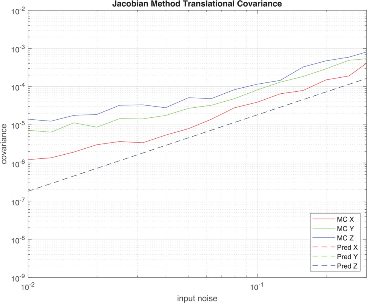
Results of Jacobian Method on a 1×2×3 box
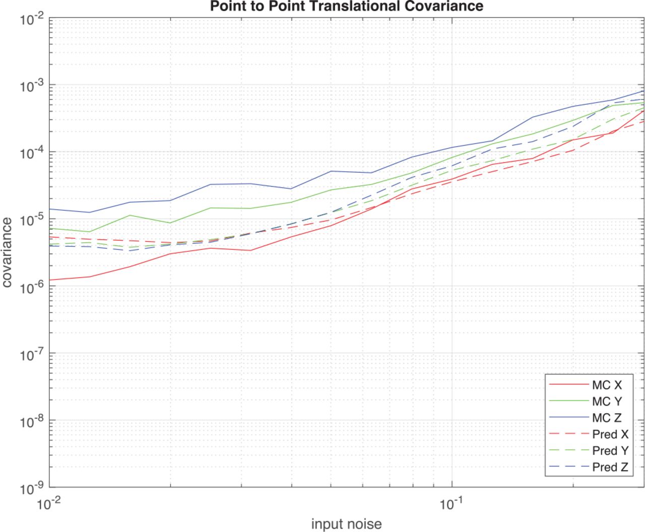
In Figures 7 and 8, we show the results of the point-to-point and point-to-plane methods from Section 2, respectively. The point-to-point method performs much better than the Jacobian method. However, it still suffers from the error case shown in Figure 3, causing it to assume information was generated in more directions than the box shape actually allows for. In aggregate, these optimistic errors combine in the extended Kalman filter (EKF) to result in an output covariance estimate that is more optimistic than the truth (Monte-Carlo estimate).

Results of point-to-point method on a 1×2×3 box

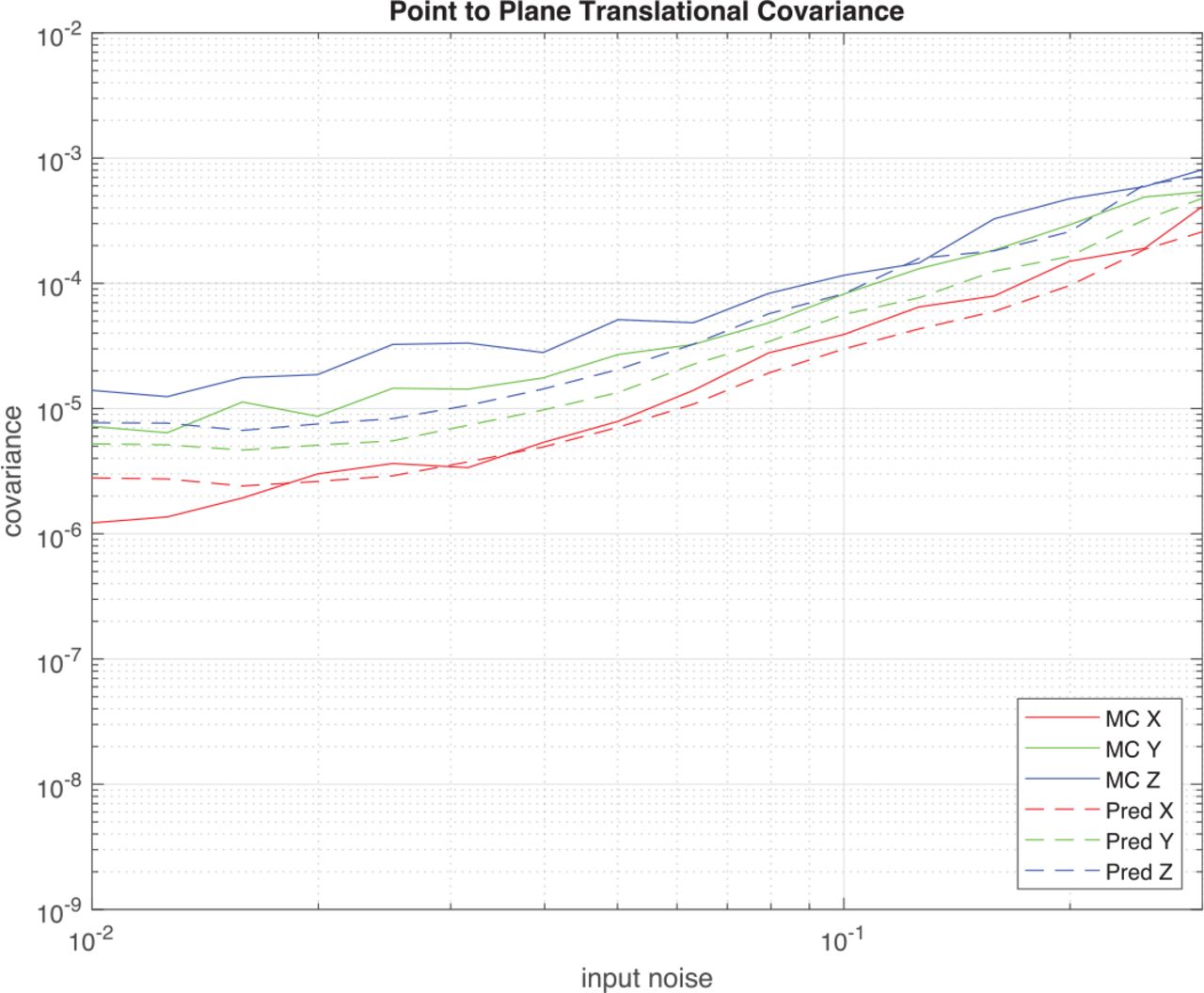
Results of point-to-plane method on a 1×2×3 box
Finally, the performance of the point-to-plane method is shown in Figure 8. By explicitly limiting the information generated by each sensed point to the vector orthogonal to the planes generated by the reference points, errors due to point mismatches and finding points between reference points can be overcome. In Figure 8, specifically note that (a) there is now significant differentiation in the predicted accuracy between points that corresponds with the size of the orthogonal planes (x has the smallest covariance, z the largest) and (b) the plot lines of MC vs predicted are significantly closer together than for either the Jacobian or point-to-point techniques. Note that the results are slightly less accurate at the lower end of the input noise range due to the noise becoming lower than the sample rate of the reference model.
To more concisely describe the closeness of plots together, we will use a new metric, the root-mean-square log error (RMSLE) for future plots. The RMSLE between predicted and MC run covariance values can be computed as:
 18
18
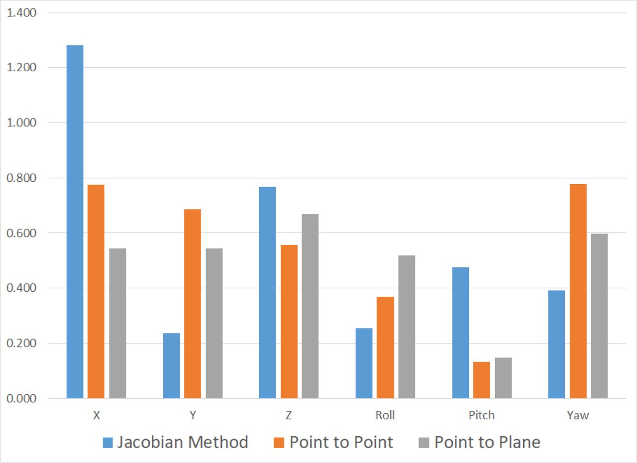
where d is the index corresponding with elements to be evaluated (e.g., X→1, roll→4, etc.), i indexes across the different noise levels of the run, MC is the Monte-Carlo covariance, and P is the predicted covariance. In this metric, a 1 would signify a 10x variance error and a 0.3 would signify a 2x variance error. Figure 9 shows the RMSLE of the three predictions on the 1×2×3 box. Using this view, it is easy identify the significant improvement in using either the point-to-point or point-to-plane method compared with the Jacobian method, and that the point-to-plane method is the overall best covariance estimator in this scenario.

RMSLE plot on a 1×2×3 box
3.2 Simulated Aerial Approach
While the previous section demonstrated that our method provided significant advantages over the Jacobian method, the way the sensed points were generated was not very realistic. To gain a more realistic evaluation of performance, in this test, the point-to-point and point-to-plane methods are applied to a simulated aerial approach of the receiver aircraft to the tanker. The simulation includes the entire vision pipeline: Cameras in the virtual world are mounted to the underside of the tanker and collect images of the receiver aircraft model; the stereo images are passed through stereo block matching to create a sensed point cloud, and the output of the stereo block matching is then fed to the ICP algorithm. Figure 10 shows an example scenario where the tanker and receiver are illustrated, together with simulated imagery in the bottom-left and -right corner of the image. The yellow dots represent the sensed point cloud generated by this system, while the red dots are the reference point cloud.

The ICP algorithm performed on simulated receiver aircraft
The receiver aircraft is initially placed 25 meters away from the camera and is moved back in 1-meter increments to a distance of 45 meters. At each position, 100 trials of ICP are run on the stereo images to create a Monte-Carlo truth covariance. To inject randomness into the simulation, a secondary point light source is moved to a random location around the tanker for each trial. In this way, the point cloud generated with each Monte-Carlo run is randomized without substantially changing the simulation parameters.
The results of this experiment are shown in Figure 11, where the RMSLE of each method is plotted. Unfortunately, no single method appears to be the best across all axes at all times. However, we still believe the point-to-plane method is best overall as:
It has no extreme errors. Note that the y-axis is on the log scale, so when the Jacobian method is off by >1.2, this corresponds to errors of more than an order of magnitude! The point-to-plane method, on the other hand, is usually less than 0.6 (a 4x variance error, or 2x standard deviation) and only exceeds this value once by a small amount.
In areas where the point-to-plane method is worse than the alternatives, the differences are generally small (and lower on the log scale) than some of the differences in the other direction. For example, when compared with the point-to-point method, the x and yaw axes both see very significant improvements in the point-to-plane methods, while the roll and z-axis results have smaller differences between the point-to-point and point-to-plane approaches.
As we show in the next section, the point-to-plane method has essentially identical performance results when compared with the state-of-the-art technique introduced in Prakhya et al. (2015).
RMSLE across various distances and lighting conditions in full AAR simulation
3.3 Prakhya vs our Method
In this section, Prakhya’s covariance estimation method (Prakhya et al., 2015)—the most applicable method from prior literature—was compared against our Kalman filter approach. This test was performed on a 1×2×3 box as discussed in the prior section, and both methods were in their point-to-plane configuration. The same method for computing normal vectors and the same input noise values were used for both algorithms.
The results show that the two estimation techniques have virtually identical predictions for the translational covariance states. The rotational states are also very similar but diverge slightly at higher input noise levels.
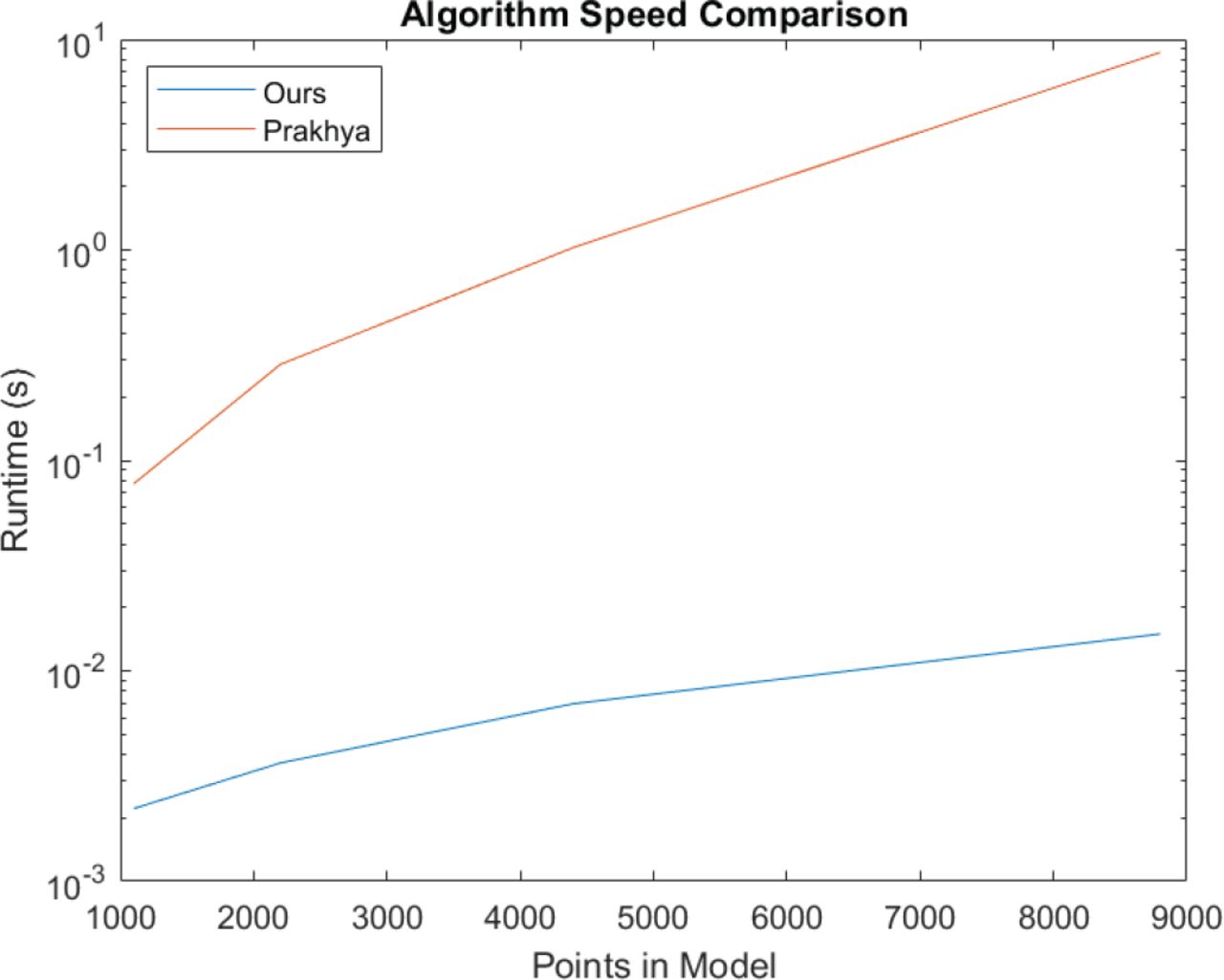
While the accuracy estimates are very similar, computationally, the requirements for these algorithms turn out to be completely different. In Figure 14, we show the runtime required to run the Prakhya algorithm vs our approach. Both methods were implemented in C++ code and on the same computer. As shown, the runtime of our approach is approximately two orders of magnitude faster than the Prakhya approach. This is primarily due to the operations on large matrices required to implement the Prakhya approach versus the the sequential processing of each point in our approach. Note that this time comparison is purely for the covariance estimation step. ICP point correspondence still takes the majority of the time in the overall loop.

Translational comparison for Prakhya vs our method on a 1×2×3 box
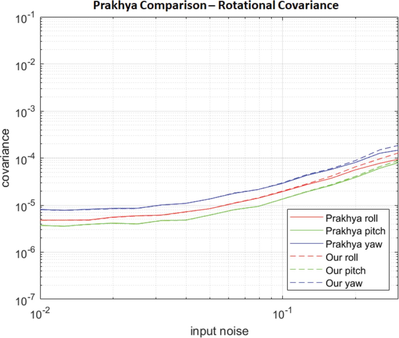
Rotational comparison for Prakhya vs our method on a 1×2×3 box

Speed comparison for Prakhya vs our method on a 1×2×3 box
3.3.1 Robustness to Sensing Conditions
In addition to being more computationally efficient, the method proposed in this paper is more robust to different sensing conditions than prior work. Because the Prakhya method relies on a fixed input noise covariance matrix that is computed a priori, its accuracy may be adversely affected by changes or degradation to the sensing scenario. Our method, on the other hand, computes the input noise values online, as described in Section 2.1, making it more robust to changing sensing conditions. To demonstrate this robustness, a 21×21 box filter was applied to simulate a degraded sensor by blurring the input images. Example sensor inputs are shown in Figure 15. A real-life analogue of this effect would be fog accumulating on the camera lenses or the camera’s focus adjusting slightly (e.g., due to vibration).

Original image vs degraded image
In Figure 16, we plot the errors from two different techniques for dealing with the blurred sensor input: (a) we utilize precomputed input noise values collected from the nominal (unblurred) AAR run, and (b) with live computation of the input noise values as described in Section 2.1. Figure 16 shows that, for the majority of the states, computing the input covariance matrix live allowed our algorithm to increase the accuracy of the output predicted covariance matrix. This test shows that computing the input covariance online increased the robustness of the covariance estimate while reducing the calibration requirement of the computer vision pose estimation system, representing a significant improvement over prior work.
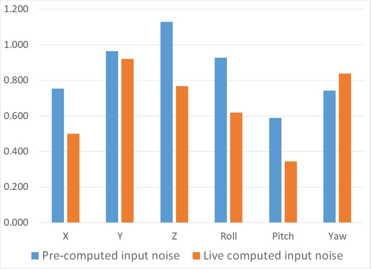
Comparative results when sensor has degraded
4 CONCLUSION
This paper introduces a novel method to estimate the covariance matrix of an ICP pose estimation problem. This approach uses the EKF update step to consolidate the information generated by each point in the sensed point cloud with each point being treated as a scalar measurement against its local surface normal vector. While this paper does not address some known shortcomings of prior methods, particularly the assumption that the ICP algorithm converged to the best solution, this method can accurately estimate the covariance matrix of the 6d pose more rapidly and with more intuitive appeal than prior methods.
This method was tested against Monte-Carlo simulations of a basic shape as well as on a fully simulated stereo vision application of automated aerial refueling. Results show that, of the two methods introduced, the point-to-plane method consistently is the better predictor of ICP covariance. Compared against the existing method by Prakhya et al. (2015), this approach produced near-identical covariance estimations while achieving a runtime improvement of over two orders of magnitude.
In this approach, the input sensor covariance is recreated from error statistics of the measured point cloud so that no information about the sensor setup is needed prior to computation. This creates a self-tuning effect, reducing the characterization load, and making the system robust to sensor degradation
For future work, a full sensor fusion application of automated aerial refueling can be implemented using the covariance matrix from this method. More generally, this ICP covariance estimation method can be directly applied to point clouds generated from other sources such as lidar, structured light, or 3D scanners.
HOW TO CITE THIS ARTICLE
Yuan, H. R., Taylor, C. N., & Nykl, S. L. (2023). Accurate covariance estimation for pose data from iterative closest point algorithm. NAVIGATION, 70(2). https://doi.org/10.33012/navi.562
Footnotes
↵1 The literature on efficiently executing ICP, navigating using ICP, applying ICP-based algorithms to different robotics scenarios, and many other aspects of ICP is extensive and beyond the scope of this paper, though a recent survey of some such topics can be found in Kolhatkar and Wagle (2021).
This is an open access article under the terms of the Creative Commons Attribution License, which permits use, distribution and reproduction in any medium, provided the original work is properly cited.


Jump to section
Related Articles
Cited By...
- No citing articles found.