

Abstract
To understand the error sources present in inertial sensors, both the white (time-invariant) and correlated noise sources must be properly characterized. To understand both sources, the standard approach (IEEE standards 647-2006, 952-2020) is to compute the Allan variance of the noise and then use human-based interpretation of linear trends to estimate the separate noise sources present in a sensor. Recent work has sought to overcome the graphical nature and visual-inspection basis of this approach leading to more accurate noise estimates. However, when using noise characterization in a filter, it is important that the noise estimates be not only accurate but also conservative, i.e., that the estimated noise parameters overbound truth. In this paper, we propose a novel method for automatically estimating conservative noise parameters using the Allan variance. Results of using this method to characterize a low-cost MEMS IMU (Analog Devices ADIS16470) are presented, demonstrating the efficacy of the proposed approach.
1 INTRODUCTION
Inertial navigation systems (INSs) provide important information about the attitude and kinematics of objects, including land, sea, air, and space vehicles. The shift toward greater vehicle autonomy and the need for accurate estimates of sensor uncertainty for sensor fusion relies on the accurate characterization of sensor errors (Hidalgo-Carrió et al., 2016; Song et al., 2011; Yuan et al., 2012). Sensor noise consists of many superposed stochastic processes that distort the measured sensor output. It is critical to measure inertial sensor noise a priori (and in some applications, online; (e.g., Song et al. [2011] and Yuan et al. [2012]) for a working INS solution due to the need to fuse inertial measurement unit (IMU) information with sensors to improve knowledge of system state. An accurate, practical, and robust characterization process is a prerequsite for optimal solutions.
Relying on manufacturer datasheets can be problematic due to faulty or incomplete noise characteristic descriptions. In addition, a datasheet can only provide approximations for a type of sensor, but not for a specific sensor. Therefore, methods that characterize a specific sensor should be utilized for more accurate covariance estimates.
Furthermore, for many navigation applications, the covariance estimate output by a Bayesian estimator may be used to determine safety-of-life or other critical navigation decisions. In these cases, the uncertainty output of the estimator must overbound or be conservative compared to the true uncertainty of the estimate. Otherwise, critical decisions about safety (e.g., can two aircraft fly next to each other with a less than 1E-6 probability of intersection) may be incorrectly decided. One way to ensure conservative output covariance is by overbounding the covariance of all input distributions (e.g., Langel et al. [2020]). In particular, the covariance estimates should overbound the true covariance for all timescales/frequencies.
Current characterization methods, however, are designed to generate noise coefficient estimates as close as possible to truth without distinguishing positive versus negative error, which disregards the risk of underestimation. This paper is motivated by the need for a calibration process that is both accurate and conservative.
Many methods have been applied for sensor noise characterization. Most ubiquitous in the navigation community are Allan variance-based methods (Allan, 1966; El-Sheimy et al., 2007; Hou, 2004; Jurado et al., 2019; Song et al., 2011; Yuan et al., 2012) including adoption as the IEEE standard for sensor characterization (IEEE, 1998, 2006, 2021). These standards describe what is referred to in the literature as the Allan Variance Slope Method (AVSM). However, because the different types of noise are additive, Allan variance plots often obscure weaker noise sources that cannot be properly estimated by the AVSM. Furthermore, as shown in Guerrier et al. (2016a), the AVSM is not a consistent estimator except in very simplistic scenarios. Therefore, recent research has suggested autonomous methods for identifying noise coefficients that do not rely solely on slope-matching. The Autonomous Regression Method for Allan Variance (ARMAV; Jurado et al., 2019) overcomes issues with the AVSM by performing a nonlinear regression in the log domain. In a more general approach, the Generalized Method of Wavelet Moments (GMWM), published in Guerrier et al. (2013) and Stebler et al. (2014) and further analyzed in Guerrier et al. (2020), suggests that optimizing in the linear, rather than log domain, leads to more accurate results.
While both ARMAV and GMWM use a least-squares optimization procedure to generate the best point estimate of Allan variance noise coefficients, to our knowledge, this paper is the first to address the estimation of conservative noise parameters from an Allan variance. The primary contribution of this paper is a modification to prior least-squares optimization procedures to ensure they produce conservative estimates of noise coefficients for a particular sensor. For this paper, we define the estimates as conservative if they are greater than or equal to the true Allan variance at all timescales. The proposed modifications are a combination of Equation (1), using the χ2-distribution to generate a 95% confidence Allan variance upper bound, and Equation (2), applying a constraint to the optimization to ensure the resultant statistics are a conservative estimate (overbound) of the additive noise sources.
The remainder of this paper is organized as follows. Section 2 provides background on the Allan variance and prior methods used for sensor characterization, namely the AVSM, ARMAV, and GMWM. Section 3 describes the approach we suggest to produce conservative noise estimates and overbound true Allan variance values. Section 4 uses the results of a Monte-Carlo simulation to compare the ability of modified and unmodified ARMAV and GMWM to tightly bound measured noise coefficients over prior methods. Furthermore, results from repeatedly characterizing an Analog Devices ADIS16470 IMU further demonstrate the need for conservative estimates. Finally, concluding remarks and a discussion of future work are given in Section 5.
2 BACKGROUND
To provide the necessary background for our proposed method, in the following subsections, we briefly review: (1) how an Allan variance is computed and the error models used to represent the sampled variance, and (2) three different techniques that can be used to estimate the error model for a given Allan variance estimate.
2.1 Error Modeling
Because the output of inertial sensors are usually fused with other sensor measurements to create a complete navigation system, characterizing the uncertainty associated with an inertial measurement is critical to the proper functioning of the fusion algorithm. Manufacturer specifications are often incomplete with only white and bias instability noise coefficient estimates (Analog Devices, n.d.; Hidalgo-Carrió et al., 2016) and inaccurate due to manufacturing tolerances and varying test conditions (El-Sheimy et al., 2007). This creates the need for an easy, reliable sensor calibration procedure.
For a general system of true state, x, and sensor measurements, z, the relationship between the actual and observed state is given by:
 1
1
where H is the observation model matrix with additive noise ϵ. In this paper, we are specifically interested in characterizing ϵ.
Several methods have been proposed for characterizing inertial sensor errors Guerrier et al., 2020; Miao et al., 2015; Song et al., 2011; Stebler et al., 2014). The use of the Allan variance has remained the active IEEE standard for calibration of both ring laser gyroscopes (IEEE, 1996, 2006), and interferometric fiber optic gyroscopes (IEEE, 1998, 2021) for several decades. The Allan variance was originally developed to characterize atomic clock stability (Allan, 1966), but since then, has found applications in a variety of contexts involving the estimation of signal noise. It is now often applied to gyroscopes and accelerometer data to estimate noise terms for modeling sensor error, providing critical information for INS solutions. The theory behind the Allan variance and methods for its computation are plentiful throughout current literature (El-Sheimy et al., 2007; Hidalgo-Carrió et al., 2016; Hou, 2004; Howe et al. 1981; Jurado et al., 2019; Vagner et al., 2012), so the discussion here will include only a short description of the connection between the Allan variance and the autocorrelation function, the essentials for computation, and brief descriptions of each noise source.
2.1.1 Allan Variance
The Allan variance uses a two-sample variance, cluster sample technique to assess the long-term performance of rate signals (Howe et al., 1981; Tehrani, 1983). The autocorrelation of a discrete signal represents the statistical dependency of a signal, x[k], with a time-shifted copy of itself. Assign the quantity:
 2
2
where n is any integer and Cov computes the covariance between the two signals. The autocorrelation of the signal x[k] will be:
 3
3
while the power spectral density (PSD) of the signal will be the discrete time Fourier transform of the autocorrelation function.
To understand the Allan variance, we first define the average of a set of samples as:
 4
4
where n is the size of the set of samples to be averaged.
The Allan variance  can be obtained as a function of the auto-correlation function using the formula (from Zhang [2008]):
 5
5
where ρ is defined in Equation (3), n is the size of clusters being analyzed, and  .
.
If the autocorrelation values, ρ(τ), are unknown, the Allan variance of a time series with N samples can also be directly estimated as:
 6
6
where m = [ N / n].
Typically, the Allan variance is plotted against τ, where τ = nΔt and Δt is the sampling time of the discrete signal (i.e.,  where fs is the sampling frequency). Note, that if N samples were collected, then
  .
.
2.1.2 Error Models
Once the estimated Allan variance is computed from samples, an explanatory model of the Allan variance data must be created. The sensor is characterized when an explanatory model that matches the errors in the collected samples is developed.
Different models have been proposed to model the error characteristics of inertial units. One model, proposed in Xing and Gebre-Egziabher (2008), models all noise as either white or non-white, where the non-white portion is modeled by a first-order Gauss-Markov process. Generally, however, more detailed structures have been used to model noise (e.g., Titterton et al. [2004]).
The more standard approach models the Allan variance as a combination of five different noise sources: quantization noise (nq), random walk noise (nrw), bias instability noise (nb), rate random walk noise (nrrw), and rate ramp noise (nrr). Because the sources are assumed to be independent, the total Allan variance is defined as the sum of variances due to these five error mechanisms (IEEE, 1996, 1998, 2006, 2021),
 7
7
Each individual noise source has a different relationship with the Allan variance as shown in Table 1.
Sources of Noise With Associated Allan Variance (AV) Slopes
To create the error model from an Allan variance plot, we describe three main techniques that have been used in the past in the following subsections. These are (a) the Allan Variance Slope Method (AVSM), (b) the Autonomous Regression Method for Allan Variance (ARMAV), and (c) the Generalized Method of Wavelet Moments (GMWM).
2.2 Allan Variance Slope Method
Until recently, the AVSM was the sole method of evaluating the strength of noise mechanisms using Allan variance data. Despite its shortcomings (Vagner et al., 2012; Hidalgo-Carrió et al., 2016) and the introduction of alternative approaches (Guerrier et al., 2020; Jurado et al., 2019; Miao et al., 2015; Song et al., 2011; Stebler et al., 2014; Yuan et al., 2012), the AVSM has maintained a continual presence in research and must be well understood before considering alternate methods.
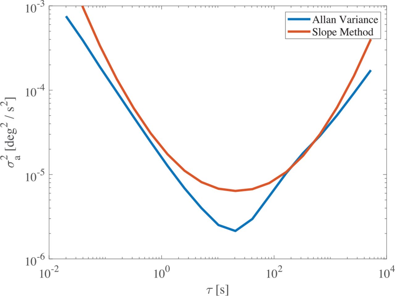
Plotting  versus τ on logarithmic axes, each of the error mechanisms in Table 1 give rise to a particular slope. The basic concept behind the AVSM is to find a portion of the Allan variance chart that is predominately one of the slopes in Table 1. That line is then extended to a specific point (the τread in Table 1) in the chart where the value associated with that noise source can be read.
In Figure 1, we show a typical result using the AVSM. The blue (lower) plot is the estimated Allan variance computed from samples of an Analog Devices ADIS16470 IMU. While the AVSM seems to perform well when each respective error mechanism slope appears in the plot, it tends to overestimate coefficients when those slopes are not present. (For example, in Figure 1 note the exceptionally steep slopes for small and large τ where the slope method overbounds the truth. This exhibits an over-estimation of quantization and rate ramp noise.) Furthermore, as shown in Guerrier et al. (2016a), the AVSM is not a consistent estimator except in very simplistic scenarios. The AVSM is also undesirable in modern applications due to inconsistent slope matching and lack of autonomy, especially when there is limited data available.

AVSM model fitted to Allan variance data. The estimated noise coefficients (generally) bound truth, but the overestimation is not a tight overbound.
2.3 Autonomous Regression Method for Allan Variance
Recent autonomous methods have been developed to increase estimation accuracy, reduce computational cost, and remove the potential need for human intervention when computing an error model for an IMU. Instead of force-fitting lines to potentially erratic Allan variance curves, ARMAV utilizes least-squares nonlinear regression to iteratively converge on an accurate overall noise characterization (Jurado, n.d.a; Jurado et al., 2019).
Let the Allan variance,  , and its associated clustering times, τ, be denoted by:
 8
8
 9
9
where N is the number of points in the Allan variance data set. The goal of ARMAV is to find the set of squared noise coefficients:
 10
10
such that the five-element noise model closely matches the estimated Allan variance for the sensor.
More specifically, the ARMAV uses a non-linear regression technique to minimize the quantity:
 11
11
where X is linear regressor matrix  using elements from the vector τ:
 12
12
and lg(·) is the base-10 logarithm:
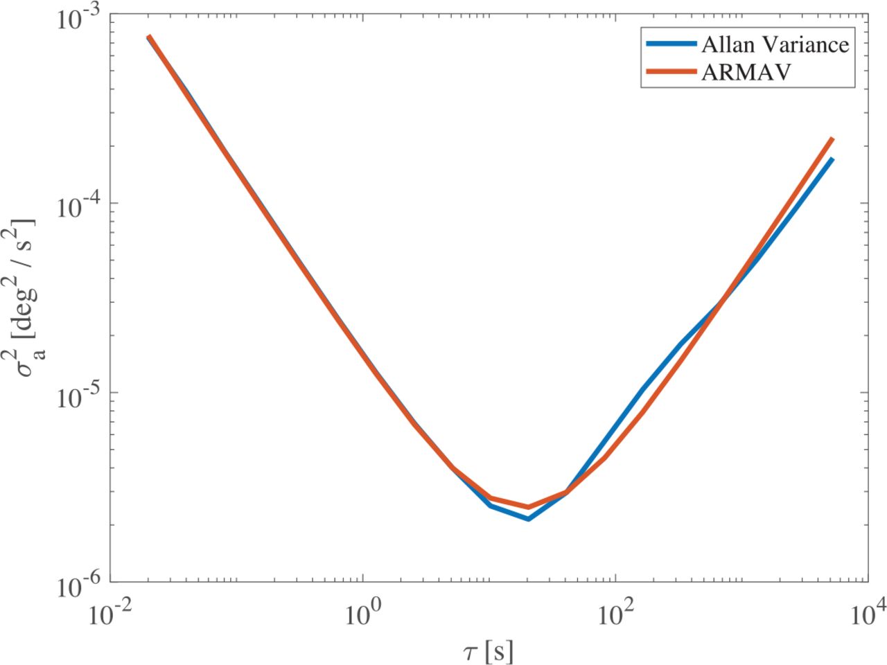
In Figure 2, the results of using the ARMAV are shown. Comparing Figure 1 with Figure 2, it is clear that the ARMAV much more closely matches the measured Allan variance curve than models using the AVSM. This translates to more consistent and accurate noise coefficient estimates and prevents overestimation of weak noise sources, substantiated by simulation results in prior work (Jurado et al., 2019), which makes the ARMAV more accurate, robust, and autonomous than the AVSM.

ARMAV model fitted to Allan variance data: This fit was generated using an unconstrained nonlinear regression (Equation [11]) using scipy.optimize.
Further improvements to the ARMAV can be made by including a weighting matrix in the cost function (Equation [11]). The weighting matrix is derived from the estimated standard deviation of the percentage error as introduced in (Jurado (2019); Equation [13]) This term is squared and inverted for each Allan variance entry to create the weighting matrix.
2.4 Generalized Method of Wavelet Moments
In Guerrier et al. (2016a, 2016b) a more general method—the Generalized Method of Wavelet Moments (GMWM)—for computing the error models from a time series of samples is introduced. The first generalization stems from the realization that the computation of the Allan variance (Equation (6)) can be represented as the computation of variance for the Haar wavelet at different timescales. The GMWM method introduces the idea of computing the variance of other wavelets to allow for alternative intermediate representations of the time-series signal. Once the intermediate representation is selected (e.g., the Allan variance or the variance of some other wavelet), a second generalization is introduced in the optimization function that maps error models to the intermediate representation. Both the AVSM and the ARMAV optimize over a function (lg(·)) of the intermediate representation, but any function can be used (including the identity function).
In later work (Guerrier et al., 2020), the ARMAV and GMWM were compared but the GMWM was limited to (a) assuming the Haar wavelet (i.e., Allan variance) and (b) using the identity function in the optimization procedure. More formally, the GMWM cost function (Equation [11]) was:
 13
13
with X as defined in Equation (12) and Ω is a weighting matrix for the different entries of Allan variance. For this paper, we use the weighting matrix defined in Jurado et al. (2019). In Guerrier et al. (2020), results were presented showing this version of the GMWM was not only at least as accurate as the ARMAV and the AVSM, but had significantly less variance in its results as well.
3 METHODOLOGY
While the GMWM and the ARMAV (best fit methods) provide significant advantages over the standards-based AVSM technique, they both have some weaknesses that we seek to overcome. First, best fit techniques do not constrain the optimization problem, so there is no guarantee of an overbound of the Allan variance for all clustering times. For example, consider the fit derived by the ARMAV shown in Figure 2. At τ ≈ 102, the Allan variance from sample data is higher than the model derived by the ARMAV. In fact, for any least-squares fit, there will always exist observation times where the modeled Allan variance falls the below measured Allan variance. This leads to estimates of the noise in inertial sensors that is less than the truth (i.e., not conservative). For safety-of-life navigation tasks or when a conservative noise estimate is otherwise desirable, the previous best fit methods are limited in their ability to provide users with confidence in the fidelity of calculated coefficients.
Second, best fit methods attempt to fit an Allan variance curve derived from a single (hopefully large) sample set. Unfortunately, there is no guarantee that, if the same sensor were used to collect another set of sensor data, the curve would not vary and be higher in some places than the current sample data. Therefore, if a conservative estimate of noise terms is desired, the probabilistic characteristics of the estimated Allan variance must be considered. We address both these issues in the following subsections (in reverse order).
3.1 Bounding Allan Variance Using the χ2-Distribution
To establish statistical bounds on the estimated Allan variance data, note that each point in the Allan variance curve is a variance computed from k samples, where k is dependent on the clustering time, τ. Therefore, we can use properties of the χ2 distribution to generate an upper bound that is guaranteed (to some probability level 1 – α, assuming the samples from which the Allan variances are estimated are normally distributed) to bound the true Allan variance. To avoid confusion between the estimated Allan variance,  , and the true population variance,
  , here we adopt the convention of
  as the calculated Allan variance (i.e., sample variance) with truth σ2.
Given a distribution of sample variance, s2, population variance, σ2, and k – 1 degrees of freedom, the chi-square statistic is given by:
 14
14
The number of degrees of freedom, k – 1, for an Allan variance data set equals the number of clusters minus one, or  for
for  .
.
Using the probability:
 15
15
we have:
 16
16
or equivalently:
 17
17
For our proposed technique, we seek to find an overbound of the additive noise. Thus, a lower one-sided (1 – α) × 100% confidence interval according to:
 18
18
is applied. Therefore, for a 95% confidence interval (α = 0.05), the least upper bound of:
 19
19
is used in place of the Allan variance point estimate, s2. In Section 4, models will be generated against this upper bound with and without an optimization constraint.
A Monte-Carlo simulation was performed to show the calculation described above, indeed, results in bounding 95% of truth Allan variance. True noise coefficients were selected to approximate a low-quality IMU and synthetic sensor data was generated (Jurado, n.d.b; Jurado & Raquet, 2017). The Allan variance for each set of simulated data was computed. For each trial, the proposed 95% confidence upper bound was also computed by taking each element of the Allan variance,  , and multiplying by the factor
  , where
  .
.
Six simulations were executed, ranging from 100 to 10,000 trials of simulated sensor data. For each trial, the discrete Allan variance points at the respective observation times were compared to the Allan variance generated from the true coefficients. The number of points that overbound the truth and the total number of points considered were added separately, and this process was repeated for every trial. Therefore, the total number of points considered for each simulation was the number of trials times the number of Allan variance points per trial of data collection (Table 2).
χ2 Simulation Results
As the number of trials increased to 10,000 (i.e., additional available sensor data), it was observed that the percent overbound of simulated Allan variance points converged to within 0.03% of the expected value. In the Figure 3(a), we show the results of 100 simulations. In the chart, the black dashed line denotes truth, and each colored line corresponds with one trial of simulated data. Approximately 50% of the data points fall below the truth value. In the second plot, the same chart is shown, but with the chi-square factor applied to each Allan variance sample. Notice that these upper bounds consistently (to ≈ 95% confidence) overbound the truth. Using this overbounding technique, we can modify the estimated Allan variance to ensure conservative uncertainty results are used by downstream fusion algorithms to weight the inertial data.

(a) Allan variance plots of simulated data against truth (b) 95% confidence upper bound of simulated data Allan variance against truth
3.2 Constrained Regression Methods
The best fit techniques the ARMAV and GMWM, apply numerical methods to solve for coefficient values subject to an error minimization objective function. To generate tight but conservative estimates of total noise, we propose to modify the ARMAV and the GMWM by adding a nonlinear constraint to the optimization to ensure the modeled Allan variance always bounds the estimated Allan variance data.
Let (Xβ)i denote the i-th element of the modeled Allan variance:
 20
20
and  denote the ith element of the estimated Allan variance, s2. Here, the objective is to solve the optimization problem:
 21
21
where f(β) is defined by either Equation (11) or (13), depending on if we are constraining the ARMAV or GMWM, respectively. Solving this constrained optimization problem results in a five-element noise model that overbounds the estimated Allan variance for all clustering times (e.g., Figure 4) and has high confidence of overbounding the Allan variance computed by another collection of the same sensor.

An example of constrained optimization using the ARMAV cost function: This model maintains a least-squares minimization, but at every observation time τ, the modeled Allan variance is greater than or equal to the measured Allan variance.
For the unconstrained problem, convergence can vary with the chosen numerical method to solve the minimization. In most cases, zeroth-order methods (e.g., Nelder Mead, Powell methods) are sufficient, typically resulting in fast solve times using only function evaluations. First-order methods, such as the Broyden-Fletcher-Goldfarb-Shanno (BFGS) algorithm, were found to require more iterations but fewer function and gradient evaluations, resulting in faster convergence time. These require the gradient of the objective function f. For the ARMAV, the derivatives of f (Equation [11]) are derived as:
 22
22
for x1 = βq, …, x5 = βrr, and assuming Ω (the weighting matrix) is a diagonal matrix.
For the GMWM, the derivatives of f (Equation (13)) are derived as:
 23
23
where Xj is the j-th column of the matrix X.
In Figure 4, we show an example of using the constrained optimization routine. While the generated Allan variance model closely matches the estimated Allan variance, it always overbounds the collected (blue) curve. In the following section, we compare the results of methods considered in this paper to demonstrate the efficacy of the constrained fit methods in generating overestimates of each noise coefficient and the total Allan variance.
4 RESULTS AND DISCUSSION
4.1 Simulation
To demonstrate the effects of the constrained optimization and chi-square overbounding techniques, a Monte-Carlo simulation of an inertial sensor with the noise characteristics outlined in Table 3 was used. The coefficients used were selected to be of comparable magnitude to an Analog Devices ADIS16470 IMU (Analog Devices, n.d.). To simplify notation, let the noise coefficients, σq, …, σrr, be given by the positive square roots of the β vector elements, namely:
 24
24
Noise Coefficients Selected for Monte-Carlo Simulation
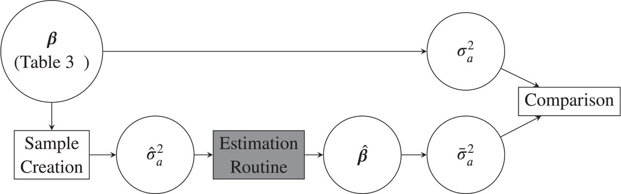
To evaluate the effectiveness of each estimation technique, we utilized the process illustrated in Figure 5. Each Monte-Carlo run consists of using the values shown in Table 3 to generate some artificial noise data with the given characteristics (the sample creation block). This was performed using a MATLAB function designed in prior work (Jurado, n.d.b) and publicly available on the Internet. Using Equation (6), the noise samples are converted into estimated Allan variance values  . The estimation routine being tested was then run to generate some predicted noise values,
  . Using Equation (12), both the true and predicted noise values can be converted into truth Allan variance values
  and predicted Allan variance values
  . The comparison of these values constitutes the rest of this section.

This figure illustrates the technique used for evaluating each estimation technique; detailed explanations of the different transitions and circles can be found in the text.
To begin, we investigate the effect of applying the weighting function to unmodified ARMAV and GMWM estimation routines. 600 different sets of data representing 1 hour of samples were generated at a 50-Hz sampling frequency. In Figure 6, we show the result of optimization for four different τ values for both unweighted and weighted versions of the ARMAV and GMWM. A violin plot of the 600 errors between the true Allan variance value and the estimated values are shown for each τ value. The τ values were chosen to be evenly spread and include the largest and smallest τ values for the simulated 1 hour of data collection.1 As shown in these figures, the weighted versions of the ARMAV and GMWM routines lead to smaller errors at all τ values, but especially the larger τ values. Therefore, all results in the remainder of this paper will be derived using weighted versions of the estimation routines.

A comparison of ARMAV and GMWM, both with and without weighting, at four different τ values: The top-left and bottom-right plots correspond with the smallest and largest τ values
In Figures 7 and 8, we demonstrate the effect of adding the constraint and χ2 overbounding to the ARMAV and GMWM estimation technique, respectively. So the magnitude of the Allan variance does not change the results, we plot the log of the ratio between the predicted and truth Allan variance values, i.e.  . Both figures show very similar results, including:
For all charts, the errors are smallest for the small τ values and increase as the τ values increase. This is expected as there are significantly more samples for small τ values.
Note that the traditional (weighted) routines significantly underestimate the true Allan variance, especially for larger τ values.
Using constrained optimization significantly increases the probability of the Allan variances being conservative. Unfortunately, there are still a significant number of values that are below the true Allan variance values.
After adding the χ2 constraint, the Allan variance values overbound the truth the majority of the time for all timescales. (More precise numbers follow.)

A comparison of the ARMAV-based weighted, constrained, and constrained with χ2 overbounding estimation techniques; the y-axis represents the values  for each given tau value (x-axis).
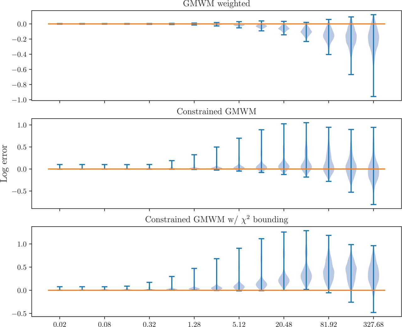
A comparison of the GMWM-based weighted, constrained, and constrained with χ2 overbounding estimation techniques. The y-axis represents the values  for each given tau value (x-axis).
In Table 4, we show the effect of the different estimation routines from data sets representing 1, 3, and 5 hours of samples. Note that the 1-hour data is the same data used to generate Figures 7 and 8. In this table, we show two different metrics for each estimation routine and set of data. The first metric (% below) is the percentage of predicted Allan variance values that are below the truth values. This metric demonstrates how effectively these routines are generating conservative predictions for the Allan variance—a fully conservative estimation routine would have 0% below. The second metric (RMSE log) returns the root-mean-squared error (RMSE), but where error is expressed as the log ratio values that were also shown in Figures 7 and 8:
 25
25
A Quantitative Comparison Between ARMAV and GMWM
where N is the total number of Allan variance samples (a product of the number of τ values for the number of hours simulated and the number of Monte-Carlo runs).
Note that many of the same lessons observed in Figures 7 and 8 can be seen again, including the necessity for both constraining the optimization and using the χ2 overbounding technique to get conservative estimates. Furthermore, we can see that less than 1% of the predicted Allan variance values will be below the truth when both of our proposed techniques are applied. One new conclusion learned from the data in Table 4 is that, after applying both modifications, the GMWM-based technique appears to have less error (its RMSE log is consistently lower than the ARMAV-based techique). Therefore, we will use the constrained GMWM with χ2 overbounding to obtain results with real data in the following subsection.
4.2 Application to Analog Devices ADIS16470 IMUs
4.2.1 Allan Variance vs. Datasheet Values
The primary motivation for this work was the need for an accurate, robust, and simple characterization process for IMUs that yield conservative estimates of sensor errors. Sensor datasheets often lack completeness of characterization and cannot be relied upon for information about different sensors, even those of the same model. In some cases, the datasheet can significantly overestimate sensor error, and in other cases, it can give underestimates, both of which are suboptimal or even dangerous in INS solutions.
To demonstrate, consider the Analog Devices ADIS16470IMU (Analog Devices, n.d.; see Figure 9). The manufacturer datasheet for this device specifies two noise parameters (excluding those that describe temperature errors and gyroscope error due to linear accelerations and vibrations): a gyro bias instability of σb = 8° / hr (2.22× 10⁻³ ° / s) and random walk error of  . The rate noise coefficient is only specified as a noise density and is restricted to a small range of frequencies (10–40 Hz). Because of this, for the datasheet Allan variance, a rate coefficient is not used in the plots that follow.

Analog Devices ADIS16470 MEMS IMU: The device footprint measures approximately 1.25″ × 1.35″.
To determine the accuracy of the datasheet noise values, 20 separate 5-hour data collections were collected from a single IMU. The Allan variance for the x-axis, y-axis, and z-axis gyros for each of the 20 static data collections were plotted against the Allan variance predicted by the datasheet values for σrw and σb in Figure 10. It was found that the datasheet values for the random walk were significant overestimates of the measured values in every case (4x variance overestimates), especially considering the strong consistency of Allan variance values at small clustering times for a given sensor axis. While it is prudent to overbound the errors to obtain conservative uncertainty estimates, this is a poor bound since it limits the usefulness of the sensor in the INS (i.e., it assumes far more uncertainty than actually exists). In addition, the lack of a random walk noise value in the datasheet leads to significant underbounding of the noise effects for times longer than about 100 seconds.

ADIS16470 comparison of datasheet (black dashed line) with measured Allan variance for x, y, and z axes: 20 runs (same sensor) of measured Allan variance are given by the thin lines.
We also show that the variation between sensors is even more significant than differences among data collection trials of the same sensor. Consider the measured Allan variances for the x-axis gyros of 12 different ADIS16470 IMUs (Figure 11). While the general trend of these data plots is roughly the same, there is significantly more deviation between sensors than there is between data corrected from a single sensor (Figure 10). Overall, this demonstrates the unreliability of using datasheet values to generally characterize a sensor model.

Comparison of Allan variances (x-axis gyro) between different sensors of the same model: Each thin line represents a different sensor, but all are of the same model (ADIS16470). This shows a greater variation than that found for a single sensor (e.g., Figure 10).
4.2.2 Noise Estimation Results With a Real Sensor
Using the 20 datasets collected from a single sensor, we apply the methods outlined in Section 3 to generate conservative noise coefficient estimates for a single sensor. First, we demonstrate the efficacy of applying constrained GMWM (CGMWM) with a chi-squared upper bound to improve confidence in an Allan variance overbound. As shown by Figure 10, there is a noticeable variation in the measured Allan variance between data sets, so it is important to consider whether the calculated coefficients for an error model also bound the results from other trials.
For every gyro axis of each data set, the original GMWM and the CGMWM against a chi-square upper bound were applied. Every predicted Allan variance point of these two models were separately compared to every estimated Allan variance point from all the other data sets from this sensor, and the fraction of model overbound points was computed for both methods. These results are shown in Table 6. Consistent with expectations, the GMWM, which is a least-squares nonlinear regression technique, achieved close to 50% overbound, while the CGMWM with chi-squared technique was conservative greater than 90% of the time. Note that this process used only the random walk, bias instability, and rate random walk noise coefficients to model the Allan variance; the quantization and rate ramp coefficients contributed little to the overall model. Sample statistics for all noise coefficients are given for all optimization methods (Table 5), including the chi-square CGMWM.
ADIS16470 Calculated Noise Coefficient Statistics: Random Walk, Bias Instability, and Rate Random Walk
Percent Overbound Between Models Generated From and the Allan Variance for 20 Data Collects of a Single Sensor
In most cases, there was a minimal increase in the coefficient magnitudes from the GMWM to CGMWM, and from the CGMWM to the CGMWM against the chi-square upper bound for the σrw terms, which is expected because the terms on the left of the Allan variance charts have so many samples that they are well characterized. On the other hand, the σrrw terms show a marked increase as the estimate routines change. This increase enables the characterized noise values to be conservative across all timescales and data collects. Although the estimated bias instability (σb) values are smaller than the values given by the datasheet, it should be noted that the estimated noise values have non-zero rate random walk values, ensuring the predicted Allan variance values overbound the true Allan variance of the sensor as shown in Table 6.
5 CONCLUSION AND FUTURE WORK
When using inertial sensors in a fusion environment, it is important that the noise be conservatively bounded. In this paper, we presented two modifications to previously published best-fit methods (the ARMAV and the GMWM) to ensure the measurements were conservative. While both the constrained ARMAV and CGMWM techniques (with χ2 overbounding) were shown to generate conservative Allan variance predictions, the CGMWM method generally had less error from the truth, making it the method of choice. These results were also shown to be more accurate than models derived from the datasheet or from any single data collection of a sensor.
For future work, note that all the data used in this paper were collected under static conditions and roughly constant temperature. As identified in prior work (e.g., Vagner et al. [2012]), thermal and vibrational noise must be controlled to generate valid Allan variance data, which directly impacts all succeeding analyses. These factors, as well as the accelerations and rotations involved in any real INS solution, must be evaluated in relation to static characterization results. Data collection should be performed to measure ground truth in a dynamic setting to evaluate sensor errors and compare against static results.
HOW TO CITE THIS ARTICLE
Lethander, K. A., & Taylor, C. N. (2023). Conservative estimation of inertial sensor error using Allan variance data. NAVIGATION, 70(3). https://doi.org/10.33012/navi.563
Footnotes
↵1 For estimating the Allan variance, τ values were chosen to range such that τ = {dt · 2j |j ∈ [1, 2, ⋯, floor(log2(N) – 3)]}, where N is the total number of samples in the data set. The −3 is used so that the largest τ values will find the variance of at least eight samples (i.e., 2j ≤ N/8).
This is an open access article under the terms of the Creative Commons Attribution License, which permits use, distribution and reproduction in any medium, provided the original work is properly cited.


Jump to section
Related Articles
Cited By...
- No citing articles found.