

Article Figures & Data
Figures
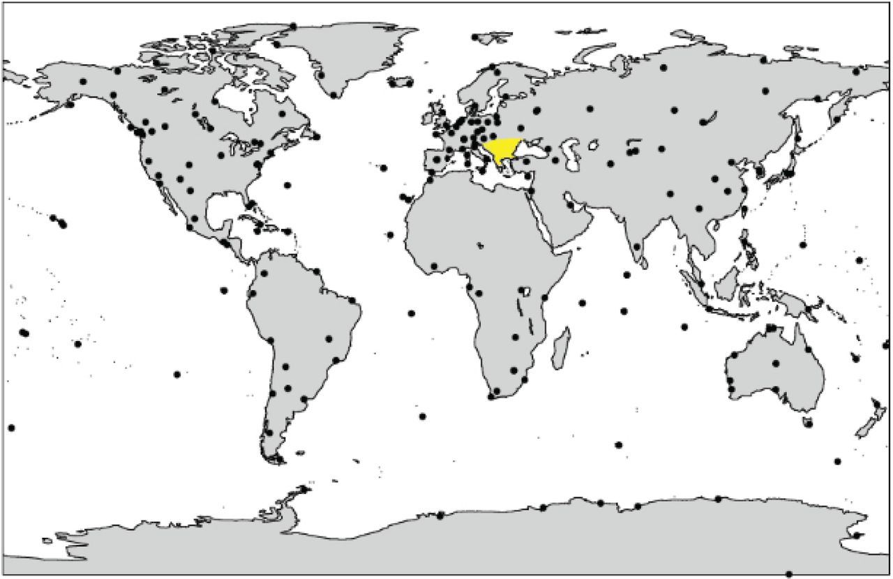
- FIGURE 1
Locations of GNSS tracking ground stations used by CODE to produce GIMs (obtained from Jee et al. (2010)).
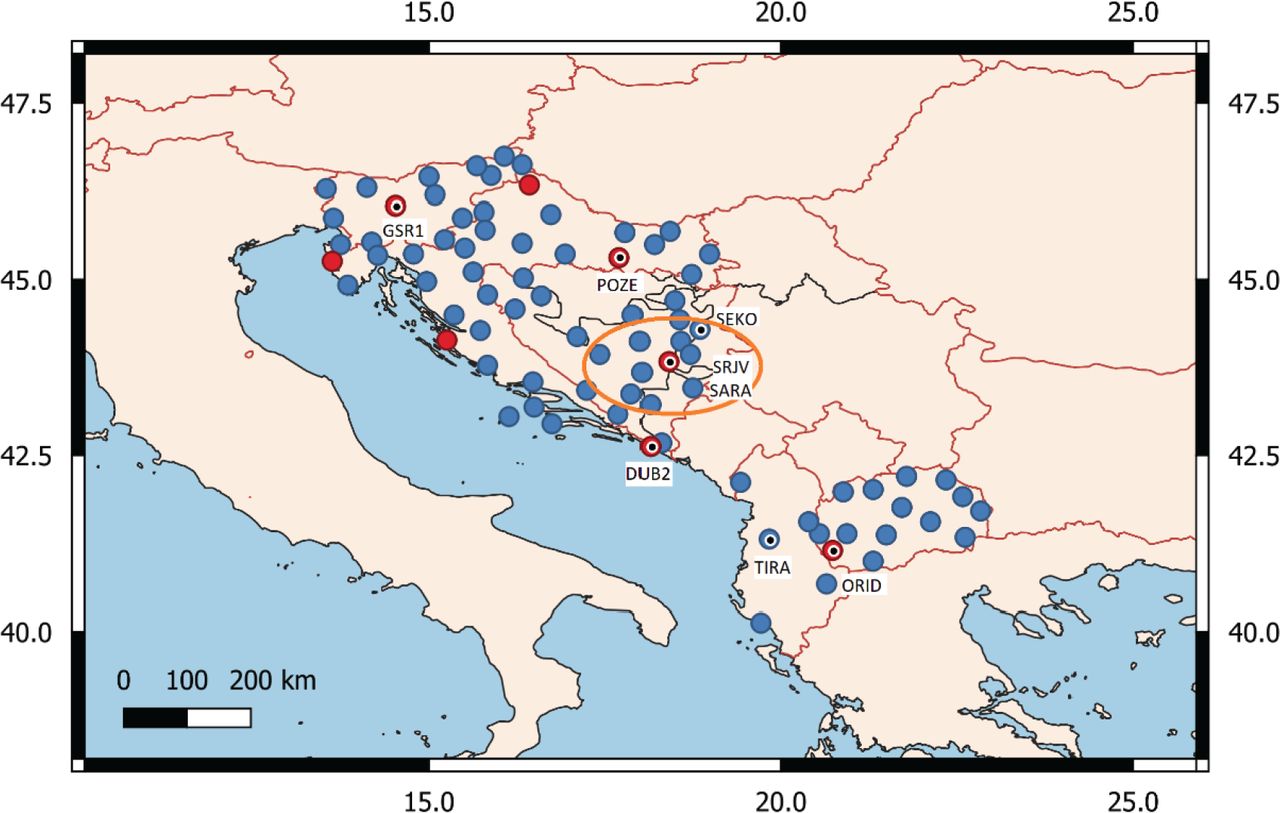
- FIGURE 2
Map documenting the locations of the dual-frequency stations of the CORS (blue dots) and the EPN (red dots) networks whose observations were used for VTEC modeling. Stations used for the RIM validation are highlighted with an inner black dot with a white rim; their names are indicated on the map.
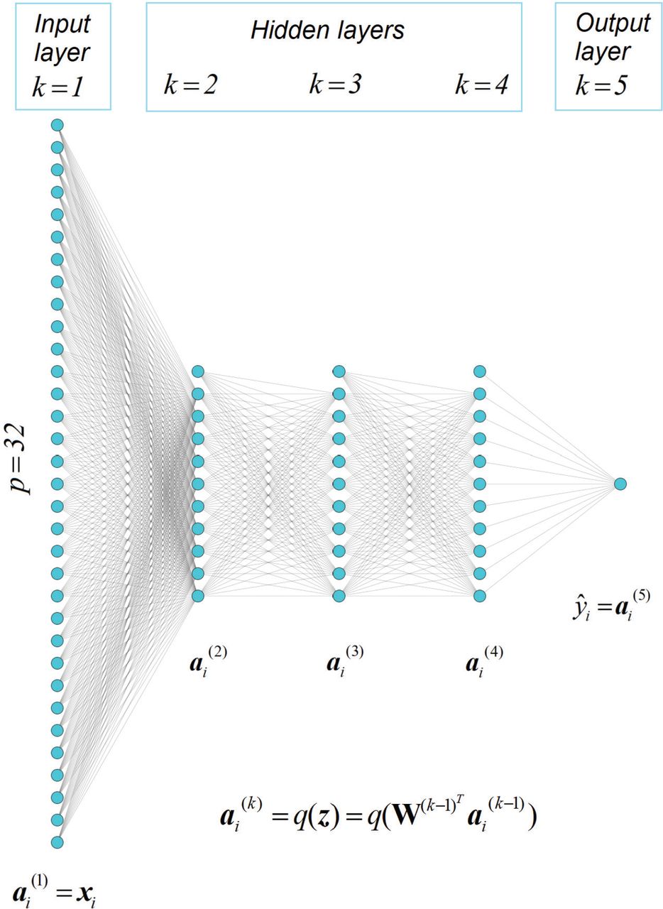
- FIGURE 3
Representation of the architecture of the ANN5 model with one input, three hidden, and one output layer (right). An additional bias unit was added to the input and the hidden layers. ANN architectures were drawn using the web-based tool NN-SVG (LeNail, 2019).
- FIGURE 4
Correlation heatmap of the input features and the output of the machine learning model.
- FIGURE 5
The RMSE (left) and correlation coefficients (CCs, right) for training and validation of ANN and RF models.
- FIGURE 6
Relative importance of input variables when training AI models with (left) and without coefficients (right) estimated using Random Forest (RF).
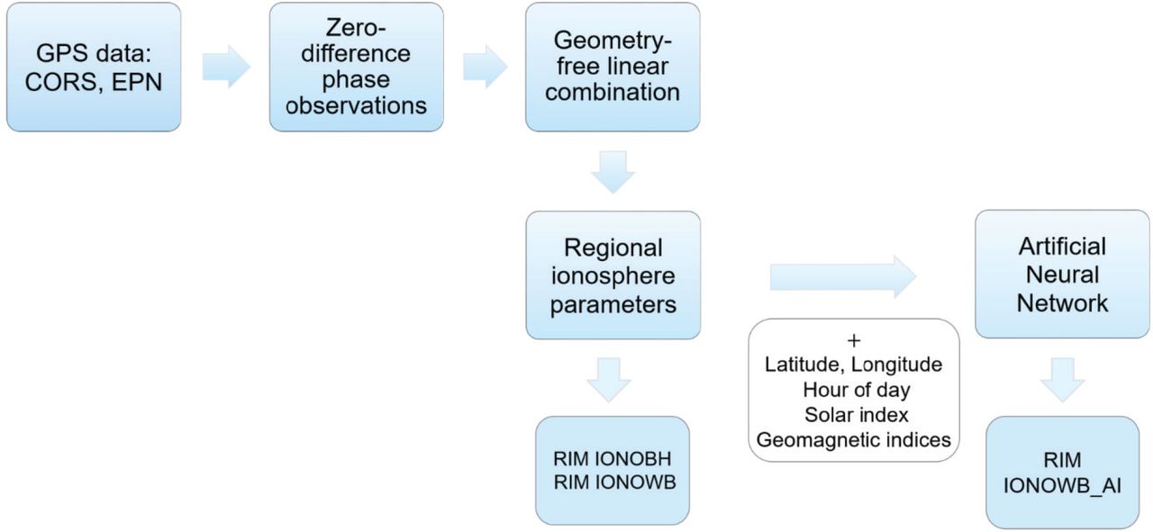
- FIGURE 7
Flowchart leading to the development of RIMs. First, GPS data from local CORS and EPN observations were processed in the Bernese GNSS software to form geometry-free linear combinations of phase observations which were then used to estimate coefficients representing the regional ionosphere parameters that form the basis of the RIM IONOBH and the RIM IONOWB. Regional ionosphere parameters were then fed into the ANN along with the spatial and temporal parameters as well as solar and geomagnetic indices, resulting in the RIM IONOWB_AI model.
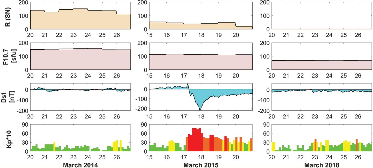
- FIGURE 8
Overview of solar and geomagnetic indices for the three study periods. Left panel: March 20-26, 2014; middle panel: March 15-20, 2015; right panel: March 20-26, 2018. From top to bottom: R sunspot number (SN), solar radio flux F10.7 in sfu (solar flux units), Dst in nT, Kp (Quiet kp · 10 < 30, Moderate 30 ≤ kp · 10 < 40, Active 40 ≤ kp · 10<50, Storm kp · 10 ≥ 50).
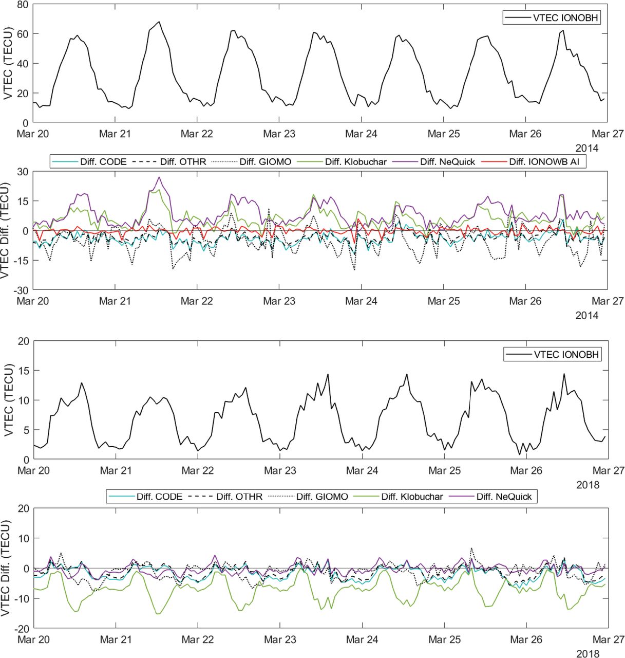
- FIGURE 9
VTEC time series and differences between VTEC from the RIM IONOBH and other models that were estimated based on the location of the EPN SRJV station. Top two panels: March 20–26, 2014 (solar maximum); bottom two panels: March 20–26, 2018 (solar minimum). Note the different scaling of the y-axes due to the effect of the solar cycle on VTEC.
- FIGURE 10
VTEC time series and differences between VTECs from the RIM IONOWB and other ionosphere models estimated based on the location of the EPN SRJV station. Top two panels: March 20–26, 2014 (solar maximum); bottom two panels: March 15–20, 2015 (includes a severe geomagnetic storm). Note the different scaling of the y-axes due to the solar cycle and the effects of the geomagnetic storm on VTEC.
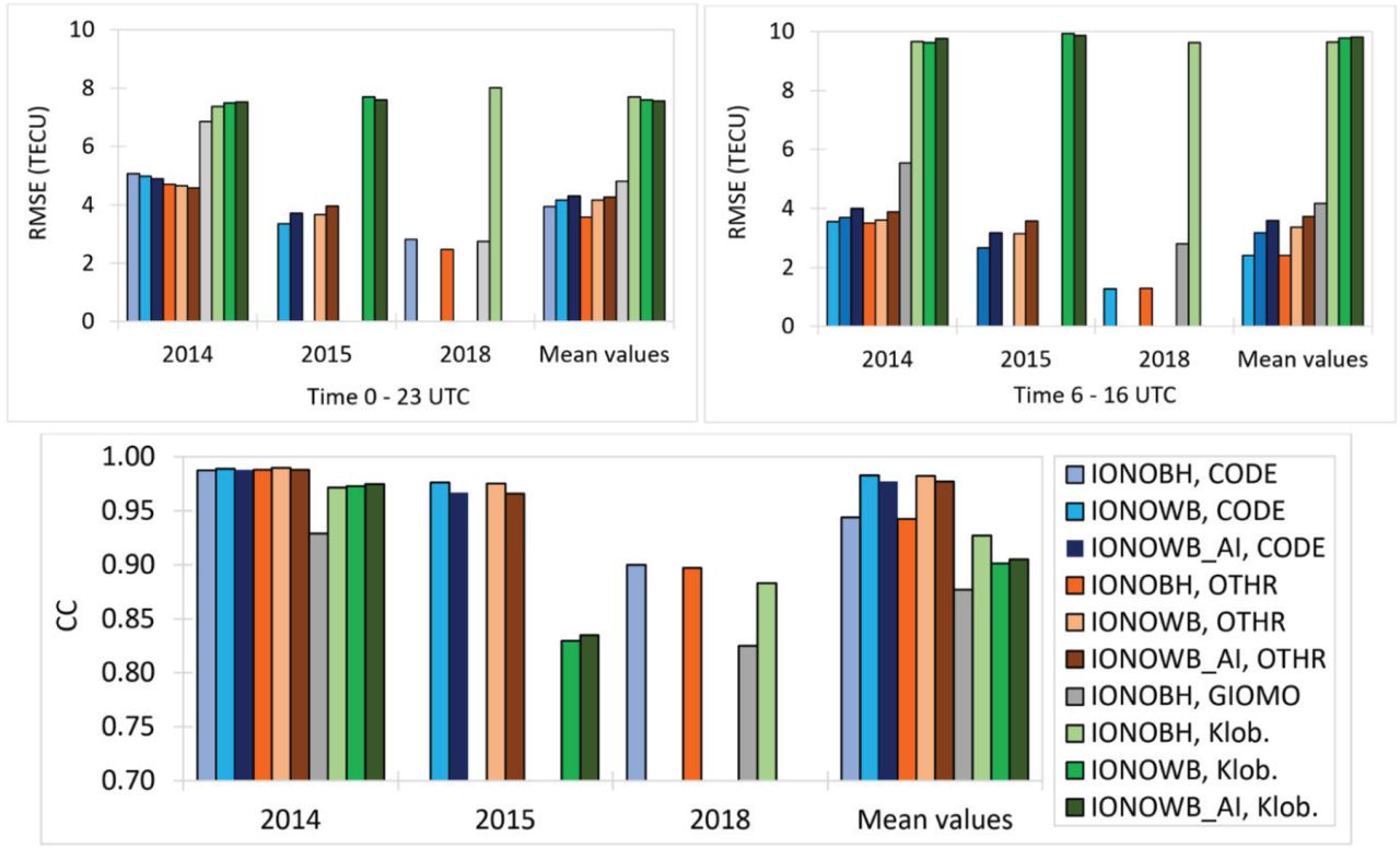
- FIGURE 11
Top: RMSE values for study periods March 2014, March 2015, and March 2018 for the entire day (0:00 to 23:00 UTC, upper left) and daytime hours only (6:00 to 16:00 UTC, upper right). Bottom: Correlation coefficients for the entire day (00:00 to 23:00 UTC). Note that correlations from 0.7 to 1.0 are shown.
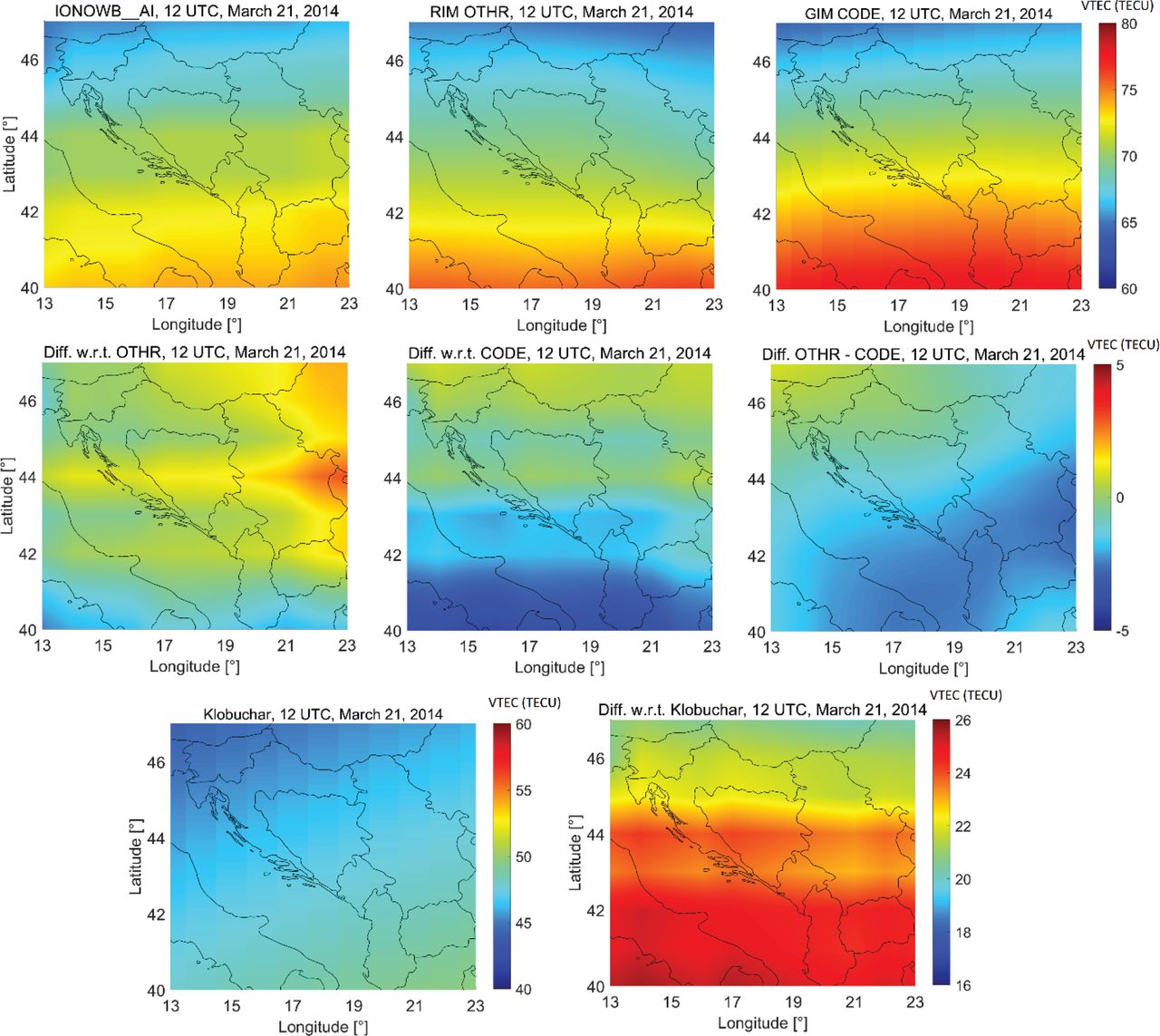
- FIGURE 12
VTEC maps (from left to right) for RIM IONOWB_AI, RIM OTHR, and GIM CODE (top). Middle: VTEC differences (from left to right): VTECIONOWB_AI – VTECOTHR, VTECIONOWB_AI – VTECCODE, and VTECOTHR – VTECCODE. Bottom: VTEC map for the Klobuchar model (left) and VTEC difference VTECIONOWB_AI – VTECKlob (right). All maps were from 12 UTC on March 21, 2014.
- FIGURE 13
VTEC maps (from left to right) for RIM IONOWB_AI, RIM OTHR, and GIM CODE (top). Mid: VTEC differences (from left to right): VTECIONOWB_AI – VTECOTHR, VTECIONOWB_AI – VTECCODE, VTECOTHR – VTECCODE. Bottom: VTEC map for Klobuchar (left) and the VTEC difference VTECIONOWB_AI – VTECKlob (right). All maps relate to 12 UTC on March 17, 2015.
- FIGURE 14
VTEC maps (from left to right) for RIM IONOWB_AI, RIM OTHR, and GIM CODE (top). Middle: VTEC differences (from left to right): VTECIONOWB_AI – VTECOTHR, VTECIONOWB_AI – VTECCODE, and VTECOTHR – VTECCODE. Bottom: VTEC map for the Klobuchar model (left) and the VTEC difference VTECIONOWB_AI – VTECKlob (right). All maps relate to 12 UTC on March 18, 2015.
- FIGURE 15
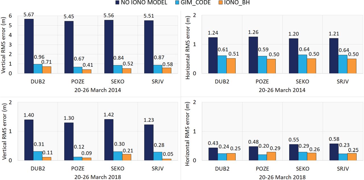
RMS errors of single-frequency positioning solutions without ionospheric corrections compared to the GIM CODE and the RIM IONO_BH. Shown are vertical position errors on March 20–26, 2014 (top left), horizontal position errors on March 20–26, 2014 (top right), vertical position errors on March 20–26, 2018 (bottom left), horizontal position errors on March 20–26, 2018 (bottom right).
- FIGURE 16
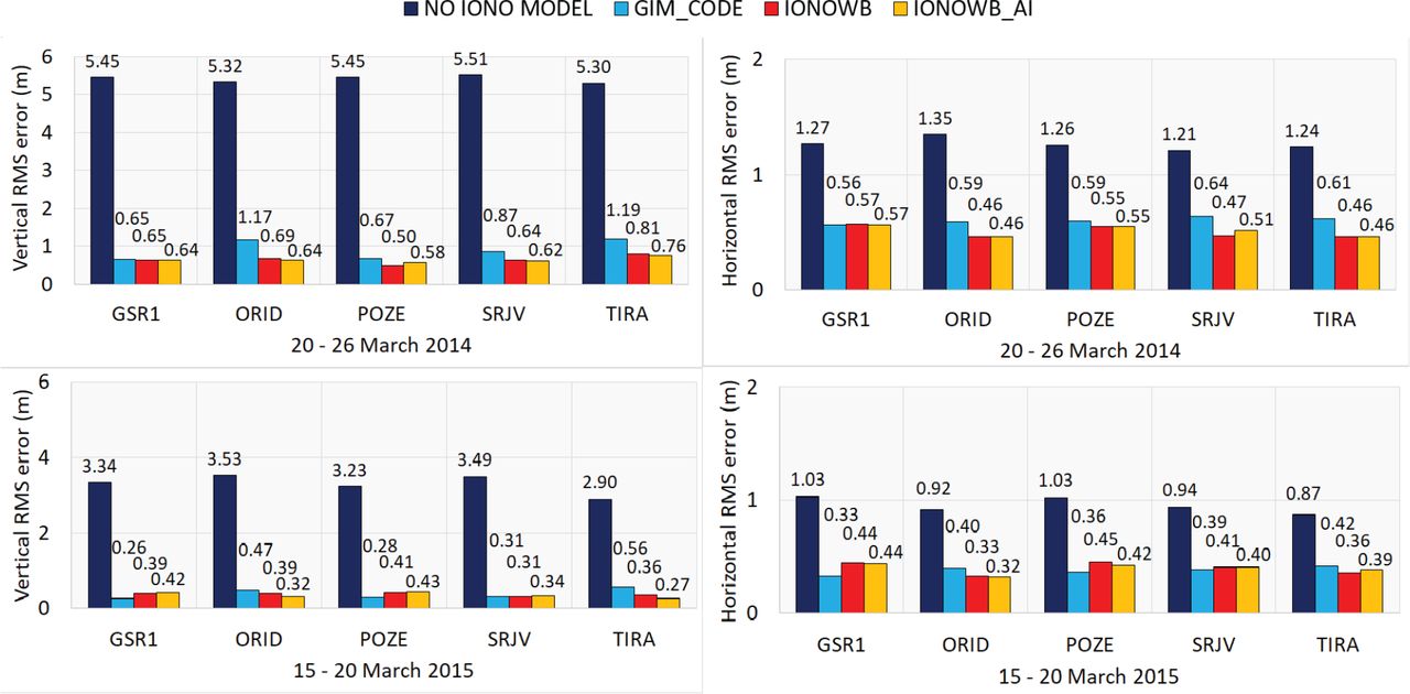
RMS errors of single-frequency positioning solutions without ionospheric corrections compared to the GIM CODE and the RIM IONO_WB. Shown are vertical position errors on March 20–26, 2014 (top left), horizontal position errors on March 20–26, 2014 (top right), vertical position errors on March 15–20, 2015 (bottom left), and horizontal position errors on March 15–20, 2015 (bottom right).


Tables
Steps Bernese software routine Cutting 24-hour RINEX observations into 1-hour files CCRINEXO Orbit and Earth’s orientation information preparation POLUPD, PRETAB, ORBGEN Satellite clock correction files preparation RNXCLK, CCRNXC Import of RINEX observation data into the Bernese format RXOBV3 Receiver clock synchronization CODSPP Ionosphere model estimation IONEST Pre-processing and processing options Linear combination for break detection (data cleaning) L4 A priori sigma of a single observation 0.01 m Elevation cut-off angle 15° Height of the single layer 450 km Degree of Taylor series expansion in latitude (nmax) 1 Degree of Taylor series expansion in hour angle (mmax) 2 - TABLE 3
AI Models with Input data, Architecture, and Training Quantities. A bias unit is added to the input and the hidden layers in the ANN. ReLu, Rectified Linear Unit, SGD, Stochastic Gradient Descent.
AI models Input data Architecture Training ANN1 Regional ionosphere coefficients
Latitude, LongitudeInput layer: 27 neurons
Output layer: 1 neuron
Linear mappingOptimizer: SGD
Learning rate: 2e-1
Momentum: 0.9
Epochs: 400
Batch size: 300ANN2 Regional ionosphere coefficients
Latitude, LongitudeInput layer: 27 neurons
Hidden layer 1: 10 neurons
Hidden layer 2: 10 neurons
Hidden layer 3: 10 neurons
Output layer: 1 neuron
Activation function: ReLUOptimizer: SGD
Learning rate: 1e-3
Momentum: 0.9
Epochs: 400
Batch size: 300ANN3 Regional ionosphere coefficients
Latitude, Longitude
HoDsin, HoDcosInput layer: 29 neurons
Hidden layer 1: 10 neurons
Hidden layer 2: 10 neurons
Hidden layer 3: 10 neurons
Output layer: 1 neuron
Activation function: ReLUOptimizer: SGD
Learning rate: 1e-3
Momentum: 0.9
Epochs: 400
Batch size: 300ANN4 Regional ionosphere coefficients
Latitude, Longitude
HoDsin, HoDcos
F10.7Input layer: 30 neurons
Hidden layer 1: 10 neurons
Hidden layer 2: 10 neurons
Hidden layer 3: 10 neurons
Output layer: 1 neuron
Activation function: ReLUOptimizer: SGD
Learning rate: 1e-3
Momentum: 0.9
Epochs: 400
Batch size: 300ANN5
IONOWB_AIRegional ionosphere coefficients
Latitude, Longitude
HoDsin, HoDcos
F10.7
Kp, DstInput layer: 32 neurons
Hidden layer 1: 10 neurons
Hidden layer 2: 10 neurons
Hidden layer 3: 10 neurons
Output layer: 1 neuron
Activation function: ReLUOptimizer: SGD
Learning rate: 1e-3
Momentum: 0.9
Epochs: 400
Batch size: 300ANN6 Latitude, Longitude
HoDsin, HoDcos
F10.7
Kp, DstInput layer: 7 neurons
Hidden layer 1: 10 neurons
Hidden layer 2: 10 neurons
Hidden layer 3: 10 neurons
Output layer: 1 neuron
Activation function: ReLUOptimizer: SGD
Learning rate: 1e-4
Momentum: 0.9
Epochs: 200
Batch size: 50RF1 Regional ionosphere coefficients
Latitude, Longitude
HoD
F10.7, Kp, DstNumber of trees= 300
Min_samples_split=5
Min_samples_leaf=3Criterion: Mean
squared errorRF2 Latitude, Longitude
HoD
F10.7, Kp, DstNumber of trees= 300
Min_samples_split=5
Min_samples_leaf=5Criterion: Mean
squared error Dataset ANN1 ANN2 ANN3 ANN4 ANN5 ANN6 RF1 RF2 RMSE
(TECU)Train 7.31 3.99 3.00 2.86 2.60 8.34 2.67 8.51 Validation 7.15 4.01 3.11 2.86 2.73 8.73 2.83 8.75 CC Train 0.906 0.974 0.985 0.986 0.989 0.876 0.988 0.870 Validation 0.910 0.973 0.984 0.986 0.987 0.869 0.986 0.868 - TABLE 5
Overview of the Mean Differences for the Solar Maximum (March 21, 2014) and the Geomagnetic Storm (March 17–18, 2015) for the Region from 13°E to 23°E Longitude and from 40°N to 47°N Latitude. Mean values from both periods (final column) were calculated based on the mean differences from March 21, 2014, and the mean differences averaged over March 17–18, 2015.
Differences between models Absolute mean differences (TECU) March 21, 2014 March 17, 2015 March 18, 2015 Mean values IONOWB_AI – OTHR 0.94 1.36 1.03 1.07 IONOWB_AI – CODE 1.48 1.40 1.05 1.35 OTHR – CODE 1.51 0.55 0.49 1.02 IONOWB_AI – Klob. 23.24 25.16 13.24 21.22 - TABLE 6
RMS errors for Vertical (ID), Horizontal (2D), and 3D Position Solutions from Static 24-hour Positioning Data. Data were averaged over all stations examined. Improvement of the RMS 3D error was observed compared to the solutions generated without ionosphere corrections.
Study periods RMS Vertical error RMS Horizontal error RMS 3D error Improvement In 3D error March 2014 NO IONO 5.46 1.25 5.49 GIM CODE 0.91 0.60 1.10 79.96% IONOBH 0.56 0.50 0.75 86.34% IONOWB 0.66 0.50 0.83 84.88% IONOWB_AI 0.65 0.51 0.83 84.88% March 2015 NO IONO 3.30 0.96 3.43 GIM CODE 0.38 0.38 0.54 84.26% IONOWB 0.37 0.40 0.54 84.26% IONOWB_AI 0.35 0.39 0.55 83.97% March 2018 NO IONO 1.34 0.51 1.45 GIM CODE 0.25 0.24 0.38 73.79% IONOBH 0.11 0.26 0.36 75.17%


Jump to section
Related Articles
Cited By...
- No citing articles found.