

Abstract
Receiver clock modeling (RCM) based on code observations requires a chip-scale atomic clock to improve the PVT solution. When using carrier phase observations, a more stable oscillator like a passive hydrogen maser (PHM) is necessary. We applied a PHM in an automotive experiment of about 80 minutes in an urban environment recording 10 Hz multi-GNSS data. Modeling the clock process noise in a linearized Kalman filter according to the spectral behavior of the PHM (i.e., RCM), improves position and velocity regarding precision and accuracy by 15% and 57%, respectively, as well as reliability by 30%. In situations with sparse, geometrically unfavorable observations, RCM prevents large position drifts. The convergence time of the carrier phase ambiguities is not affected. Conclusively, precision, accuracy, and reliability in kinematic precise point positioning can be improved by using an oscillator like a PHM. Future advancements in clock technology should make this approach more feasible for ordinary use cases.
1 INTRODUCTION
Since each Global Navigation Satellite System (GNSS) is based on one-way range measurements, single-receiver GNSS positioning, navigation, and timing applications always require the synchronization of the timescales of the receiver and the used satellites. This is usually done by introducing so-called clock biases relative to a superior GNSS timescale into the estimation process for both satellites and receiver. Corrections for satellite clock biases can be obtained in real time via the GNSS navigation message or from data distributed in real time by International GNSS Services (IGS).
For post-processing applications, more precise corrections are computed and provided by the IGS (Johnston et al., 2017) as a free-of-charge service through the internet. Regarding the receiver, the corresponding clock bias must be corrected by the user. Due to the poor accuracy and limited long-term frequency stability of the built-in quartz oscillator, this clock bias has to be estimated together with the receiver coordinates at each observation epoch. Thus, in order to determine a three-dimensional position, the user must have at least four satellites in view simultaneously.
This standard approach of GNSS-based positioning leads to further drawbacks:
a) High mathematical correlations emerge between the estimated clock bias, the up-coordinate, and other elevation angle-dependent error sources such as the tropospheric delay estimates (Rothacher & Beutler, 1998).
b) The precision of the up-coordinate is always about two to three times worse than that of the horizontal coordinates (Santerre et al., 2017).
One possibility to overcome these disadvantages is replacing the internal quartz with a more stable external oscillator, for instance, an atomic clock. In addition, the implicit clock model of the estimator applied in data analysis has to be adapted according to the superior performance of such an oscillator (Misra, 1996; Sturza, 1983). This approach, referred to as receiver clock modeling (RCM), is especially beneficial in kinematic applications as shown by Weinbach and Schön (2011) and Krawinkel and Schön (2016).
The applicability of RCM depends on the frequency stability of the oscillator and the GNSS observation type in use. This means that in applications using carrier phase observations such as precise point positioning (PPP) (Zumberge et al., 1997), RCM is only feasible if a highly stable oscillator like a hydrogen maser is used (Wang & Rothacher, 2013; Weinbach, 2013; Weinbach & Schön, 2015). On the other hand, when using code observations, meaningful RCM can be applied with much smaller but still very stable oscillators like a chip-scale atomic clock (CSAC) (Krawinkel, 2018).
In light of an increasing number of location-based services that rely on or have the need for very accurate autonomous position and velocity determination, applying RCM with carrier phase observations (i.e., PPP) is of particular interest. No oscillator currently exists that provides the required stability and is designed to be operated in kinematic applications. Nevertheless, a transportable passive hydrogen maser (PHM) could be carefully used in a dedicated test case, which would act as proof of concept in a way. Therefore, the main goal of this contribution is to assess the benefits of using a highly stable oscillator in GNSS-based navigation. This will be quantified in terms of typical performance parameters such as the precision, accuracy, and reliability of the position and velocity solution. In addition, we will also investigate the impact on the observation domain (i.e., outlier detection).
The article is structured as follows: first, we will recapitulate the basic principles of RCM focusing on implementation in a Kalman filter; this approach is then evaluated by means of an automotive experiment in which the environmental setting is described in Section 3; the data analysis and corresponding results are explained and discussed in Sections 4 and 5, respectively; and conclusively, we close the article by summarizing our most important findings.
2 RECEIVER CLOCK MODELING
The fundamental principle of physically meaningful receiver clock modeling is based on the condition that the noise of an oscillator must be smaller than the noise of the GNSS receiver it is connected to. This means that the deviations from a polynomial, typically linear clock model caused by accumulated random frequency fluctuations of the oscillator cannot in the short-term be resolved by the observations of the receiver.
The receiver noise is assessed by means of the noise of the observation type in use since this ultimately determines the precision (i.e., noise level) of the position, velocity, and time (PVT) solution. Due to their non-stationary behavior, the oscillator noise is typically characterized by time-dependent measures such as the Allan Deviation (ADEV) (Allan, 1987), which allows an easy juxtaposition with the noise behavior of the receiver.
As an example, in this case study, we assess the noise of GPS L1 C/A code and ionosphere-free carrier phase observations as 3 m and 6 mm, respectively, at an average time of 1 second. Since these are phase observations, they can be modeled as white phase noise over time. Besides conducting individual clock comparisons and calculating instrument-specific frequency stability parameters thereof (Jain et al., 2021), this information can be and is usually derived from manufacturer’s data. Note that the latter might deviate considerably from the actual oscillator behavior as shown by Krawinkel and Schön (2014). Therefore, the user has to decide from application to application whether to consider this uncertainty or not. For the more general and explanatory remarks in this section, it is sufficient to rely on manufacturer’s data. Instrument-specific parameters will be discussed later in Section 4.2.
Figure 1 shows the stated GPS observation noise curves as well as typical Allan deviations of a CSAC and a PHM as specified by the respective manufacturers (Microchip, 2020; Vremya-CH, 2020). By converting these values to so-called time prediction errors (TPE), the evolution of the time deviation of an oscillator can be computed. Since all these noise processes are assumed to be white, the computation is very straightforward, multiplying the ADEV with its corresponding average time. If the ADEV curve also exhibits types of colored noise, their time-dependent evolution has to be taken into account, too, as discussed by Allan and Hellwig (1978).

Typical Allan deviations and consequential time prediction errors of a chip-scale atomic clock (CSAC) and a passive hydrogen maser (PHM) as well as GPS L1 C/A code and ionosphere-free (L0) carrier phase observation noise modeled as white phase noise over time
From the TPE, maximum intervals of physically meaningful receiver clock modeling (RCM) can be derived by means of the intersection points between the TPE and the observation noise curves. In the case at hand, for example, RCM using a CSAC and GPS L1 C/A code observations is feasible for up to roughly 17 minutes (𝜏𝑝 ≈ 1000 s). On the contrary, applying a passive hydrogen maser (PHM) enables carrier phase-based PVT such as PPP.
The technique of RCM can be implemented in different ways depending on the estimator applied in GNSS data analysis. In a least-squares adjustment (LSA) based on GNSS observations only, the functional model is changed: the epoch-wise estimation of the receiver clock bias is replaced by a piece-wise linear polynomial, in which each segment covers an interval that corresponds at most to the theoretical maximum clock modeling interval. In order to avoid discontinuities between consecutive modeling segments, their slopes can be constrained according to the stability of the oscillator in use. This approach is applicable in both batch and sequential LSAs as shown by Weinbach (2013) and Krawinkel (2018), respectively.
A very popular method in kinematic PVT determination is the use of an extended Kalman filter (EKF) or linearized Kalman filter (LKF). Here, the functional model (i.e., the measurement model) stays unchanged, but the system model is adapted by means of the clock process noise model. Typically a two-state model representing a random ramp process of clock offset and drift is employed (Brown & Hwang, 2012):
 1
1
with the spectral amplitudes 𝑆𝜙 and 𝑆𝜈 of the oscillator phase and frequency deviations, respectively, integrated over a certain time period Δ𝑡. A more extended model can be found in Chan and Pervan (2009) and subsequent publications. The amplitudes can be described as functions of power spectral density (PSD) coefficients ℎ𝛼 each of the latter representing a specific power law process (Barnes et al., 1971; Rutman, 1978). The superposition of these processes sums up to the overall PSD:
 2
2
with the Fourier frequency 𝑓 and the intensity coefficients ℎ𝛼 each of a distinct power law exponent 𝛼. Table 1 gives an overview about the five most common power law processes and their respective exponents.
Power law processes and their characteristic exponents
Approximations of 𝑆𝜙 and 𝑆𝜈 are given, for example, by Brown and Hwang (2012) as:
 3
3
 4
4
or directly in terms of the clock process noise matrix by van Dierendonck et al. (1984):
 5
5
with:
 6
6
 7
7
 8
8
Note that the latter model was corrected by Brown and Hwang (1997) so that Equations (6) to (8) do not use the original terms but the corrected ones.
The main difference between these two models is the fact that the model by van Dierendonck et al. (1984) not only considers white frequency modulation (WFM) and random walk frequency modulation (RWFM) noise—like the model by Brown and Hwang (2012) in Equations (3) and (4)—but also flicker frequency modulation (FFM) noise. That means it is more appropriate to represent or assess, respectively, the behavior of an oscillator that exhibits significant FFM noise. Although the stability of the oscillators discussed in the following sections is dominated by mainly WFM and partly FFM noise, we will use the model by van Dierendonck et al. (1984) in our case study.
3 AUTOMOTIVE EXPERIMENT
In order to evaluate the benefits of using a highly stable oscillator in a kinematic GNSS application, an automotive experiment was carried out in the city of Hannover, Germany, on July 9, 2018. The whole test drive lasted for approximately 80 minutes and took place mainly on city streets and partly on a federal highway, thereby approaching velocities of up to 93 kilometers-per-hour. Figure 2 shows the overall trajectory.

Trajectory of the test drive within the city of Hannover, Germany, with the orange arrows indicating the driving direction. The yellow triangle represents the location of the GNSS reference station, where also the start and end point of the drive were nearby. The yellow dots illustrate locations of extended static phases of the vehicle; they partly coincide with the light blue dots indicating different points in (GPS) time of the test drive
In order to be able to investigate the impact of using a PHM in a kinematic application, different dynamics were driven in various environmental situations. This can be also seen from the velocity estimates of the reference solution shown by Figure 3 and discussed in Section 4.1. This shows that also two static phases of approximately 13 minutes each were included, serving as best case scenarios compared to the rest of the drive where the PHM was exposed to more or less pronounced dynamic stress.

Velocity estimates of the reference solution for the whole experiment
Regarding different environmental influences such as obstructions and frequent interruptions of the incoming signal, we drove through very good conditions as well as more challenging surroundings like tree-lined roads and densely developed urban areas. This also applies to both static phases, as the latter phase took place right next to a tree line.
The measurement configuration inside the vehicle as depicted in Figure 4 consisted of three high-end GNSS receivers, namely two JAVAD Delta TRE-G3T—both running the same firmware version—and one NovAtel SPAN-SE-D. Each JAVAD receiver was driven by the 10 MHz signal of a different external oscillator: a Vremya VCH-1006 PHM—provided by Physikalisch-Technische Bundesanstalt (PTB), Germany’s national metrology institute—and, for comparison, a Microsemi miniature atomic clock (MAC) SA.35m. A tactical-grade inertial measurement unit (IMU), namely the iIMU-FSAS-EI-SN from iMAR Navigation GmbH, was used in combination with a NovA-tel receiver.

Measurement configuration of the automotive experiment
The three receivers were connected to the primary antenna, a NavXperience 3G+C, via an active signal splitter. An identical secondary antenna was directly plugged into the corresponding input connector of the NovAtel receiver. Both antennas separated by about 0.95 m were mounted with the IMU on a calibrated measurement platform on the roof of the vehicle as depicted on the right-hand side of Figure 5.

Parts of the measurement equipment: on the left, passive hydrogen maser (PHM) placed inside the trunk; and on the right, an inertial measurement unit (IMU) and GNSS antennas mounted on the roof of the vehicle
The PHM, the centerpiece of the experiment, was carefully fixed inside the trunk of the car. As can be seen from the left-hand side of Figure 5, supplementary damping material was added to its transport frame to reduce the impact of external vibrations and shocks to the delicate oscillator. The power supply was ensured onboard by the vehicle itself combined with an independent battery backup.
Furthermore, a local reference station consisting of a JAVAD Delta TRE-G3TH receiver and a Leica AR25 antenna was run, with the latter permanently installed on a concrete pillar on the rooftop of the GNSS laboratory. All receivers recorded multi-GNSS observations with a data rate of 10 Hz and the IMU operated at 200 Hz.
4 DATA ANALYSIS
The validation of a given test dataset can be carried out by means of a reference solution of at least one magnitude higher precision. Therefore, this section first discusses the computation of such a reference solution of the vehicular trajectory outlined in Section 3. Subsequently, the core analysis of the recorded kinematic data set with the in-house software tool is described as well as important processing settings.
4.1 Reference solution
Since the measurement configuration consisted of both GNSS and inertial sensors, and considering the test drive took place in an urban environment with frequent signal interruptions and a lot of adverse observation geometries, a tightly coupled GNSS/INS solution was used to compute the reference trajectory for all further investigations. This was done by means of the TerraPos software, version 2.5.4, which is a state-of-the-art solution for kinematic position, velocity, and attitude determination (Kjørsvik et al., 2009; Terratec, 2020).
To be more specific, a relative positioning solution is computed using the 200 Hz IMU data combined with the 10 Hz dual-frequency GPS L1/L2, GLONASS G1/G2, and Galileo E1/E5a code, carrier phase and Doppler observations of the local reference station, and the JAVAD receiver connected to the PHM inside the vehicle. In addition, satellite orbit and clock corrections of the Multi-GNSS Experiment (MGEX) project of the IGS (Montenbruck et al., 2017) was used, provided by the Center for Orbit Determination in Europe (CODE) (Prange et al., 2020).
There are two reasons why we did not use the GNSS data of the NovAtel receiver: First, our receiver only records legacy dual-frequency GPS and GLONASS observations, which is a significant disadvantage in an urban setting like this. For instance, often GPS P2 observations are not available but modern GPS L2C are. Second, applying the same receiver type on both ends of the relative solution reduces manufacturer-specific, or in this case receiver type-specific, biases improving the overall consistency of the solution. Furthermore, an elevation cutoff angle of 10 degrees and a filter update rate of 10 Hz was applied.
The TerraPos software enabled the use of a secondary antenna, which in this case, however, did not lead to a higher quality of the trajectory solution. In two different ways, this is a result of the relatively short baseline length between both antennas. The signal availability stays virtually unchanged compared to the single-antenna case (i.e., the number of observations was the same, even in challenging situations such as driving beneath an underpass), while with regard to attitude determination, the contribution of the high-precision IMU data outperformed that of the GNSS baseline link. This means that the difference between a solution with and a solution without using data of the secondary antenna was almost non-existent.
As a result, the reference trajectory exhibited a high precision for both position and velocity of the vehicle. Numerically speaking, 99% of the formal position and velocity standard deviations (SD) were smaller than 0.085 m and 0.011 m/s with maximum values of 0.095 m and 0.014 m/s, respectively. This also means implicitly that—especially in an urban environment—a GNSS/INS combination will lead to a better solution compared to only using GNSS data.
4.2 Kinematic PPP
In order to investigate the impact of the passive hydrogen maser (PHM) on high-precision GNSS-based navigation, we used the PPP module of our in-house MATLAB GNSS toolbox. We will discuss the properties and various processing parameters of the software as well as how the different solutions were computed.
The PPP module is designed for both static and kinematic multi-GNSS applications. It uses a linearized Kalman filter (LKF), processing data in both forward and backward directions to calculate an optimal solution by means of a fixed-interval smoother (Gelb et al., 1974).
Similar to the reference solution, we applied ionosphere-free GPS, GLONASS, and Galileo code, as well as carrier phase and Doppler observations with an elevation cutoff angle of 10 degrees and a data rate of 10 Hz.
GPS L2C observations were used if transmitted by the respective satellite. This is especially beneficial in an urban environment because often the legacy P2 observations of the same satellite are not available due to the significantly lower signal strength compared to the modern L2C signal. The a priori observation SDs 𝜎𝑙𝑖 of the ionosphere-free code, carrier phase, and Doppler observations were chosen as 6 m, 0.015 m, and 0.1 m/s, respectively. The elements of the main diagonal of the corresponding variance-covariance matrix 𝐑 are determined by:
 9
9
based on observation weights:
 10
10
with satellite elevation angle 𝑒𝑖 of the 𝑖-th observation.
Equation (10) does not down-weight observations with low elevation angles as much as the standard approach of:
 11
11
and helps to decorrelate elevation-angle-dependent parameters such as tropospheric delay, receiver up-coordinate, and receiver clock offset. This was validated by means of two extended static periods during the experiment, each lasting for 13 minutes. Here, the root-mean-square errors (RMSE) of both the post-fit residuals and the position deviations, especially the up-component, were smaller when applying Equation (10) instead of Equation (11). Thus, the former weighting scheme is a better stochastic representation of the observations in this case.
A prerequisite for PPP is the accurate modeling and correction of numerous errors affecting observations. Besides using the same satellite orbit and clock products as in the case of the reference solution, satellite differential code biases (DCB) were accounted for by applying the corrections provided by the German Aerospace Center (DLR) (Montenbruck & Hauschild, 2013; Prange et al., 2017).
Signal delays due to tropospheric refraction were modeled by the empirical Vienna mapping function three (Landskron & Böhm, 2018). Ionospheric effects were already significantly reduced or eliminated, respectively, by forming the ionosphere-free linear combination.
GPS, GLONASS, and Galileo satellite antenna phase offsets and variations (PCO, PCV) were corrected by applying the most recent IGS14 ANTEX file at the time of processing (Rothacher & Schmid, 2010). Individual calibration values for the receiver PCO and PCV were determined by the institute (Kröger et al., 2021). Due to the lack of Galileo corrections, only GPS and GLONASS could be corrected at this point.
Nevertheless, during the experiment in July 2018, only four Galileo satellites were available, and most of the time just two or three were visible at the same time. The carrier phase wind-up (PWU) effect was modeled according to Wu et al. (1992) and refined by Beyerle (2008). Both PCO/PCV and PWU were computed relative to the actual attitude of the vehicle derived from the reference solution.
Besides the conventional relativistic correction, also the so-called Shapiro effect, a gravitational delay caused by the space-time curvature induced by the Earth’s gravity field, was corrected (Zhu & Groten, 1988). Finally, the tidal, nontidal, as well as atmospheric and oceanic loading effects were corrected according to the IERS conventions in 2010 (Petit & Luzum, 2010).
Carrier phase cycle slips were detected by comparing the geometry-free linear combination (LC) against a given threshold that depends on the wavelength of the LC and the measurement interval. In the case of detection, the corresponding carrier phase ambiguity would be reinitialized, and no attempt would be made to repair the cycle slip.
Once all necessary corrections are applied, the resulting observed-minus-computed (OMC) observations were used during each measurement update step of the LKF. Here, the total state vector at an epoch 𝑘 reads:
 12
12
with the respective Earth-centered, Earth-fixed (ECEF) position and velocity state vectors:
 13
13
 14
14
with receiver clock time offset 𝛿𝑡 and drift 𝛿𝑓, residual tropospheric zenith delay Δ𝑇, GLONASS and Galileo intersystem code biases (ISCB) 𝛿𝑡𝑅 and 𝛿𝑡𝐸, respectively, and float carrier phase ambiguities 𝑁𝑖 for each satellite 𝑖 = {1,…,𝑛} ∈ ℕ. Note that the float ambiguities also include or absorb, respectively, the GLONASS and Galileo intersystem carrier phase biases. If integer ambiguity resolution would be applied, these biases also would need to be estimated explicitly, which is not the case in this study.
Another crucial part of Kalman filtering is the proper assessment of the process noise. The dynamics of the vehicle are described by a position-velocity model assuming near-constant velocity during consecutive filter recursion steps. Since there are only small deviations from that as can be seen from the reference solution, the spectral amplitude for the position random process is assessed to 2m2/s3.
At this point, we want to make clear that this value is typically tuned from application to application. In this case, however, we chose a rather relaxed value since emphasis in our analysis was put on the impact of using different spectral coefficients/amplitudes for the receiver clock noise process. The velocity noise process is derived thereof according to Brown and Hwang (2012).
The receiver clock offset and drift are modeled as a random ramp process as proposed by van Dierendonck et al. (1984) [see Equations (5)–(8)]. In addition to the coefficients corresponding to the Vremya PHM and the Microsemi MAC, also those of a typical temperature-compensated crystal oscillator (TCXO) are considered. The latter is then referred to as a solution without RCM, because the user oftentimes does not know about the type of oscillator onboard the receiver.
In addition, when using commercial GNSS software, it is usually not possible to apply specific clock PSD coefficients, let alone be able to alter the clock model itself. Thus, in case the PHM values listed in Table 2 and shown by Figure 6 are applied, we label it a solution with RCM. The conversions between spectral coefficients and Allan deviations are carried out according to Barnes et al. (1971):
 15
15
 16
16
 17
17

Allan deviations of the Microsemi MAC SA.35m and a Vremya VCH-1006 passive hydrogen maser (PHM)—corresponding to spectral coefficients in Table 2—as well as GPS L1 C/A code and ionosphere-free (L0) carrier phase observation noise modeled as white phase noise over time
Spectral coefficients of oscillators as used during data analysis: *derived from manufacturer’s data, †individually determined by Jain et al. (2021), ‡according to Brown and Hwang (2012)
The residual tropospheric zenith delay needs to be taken into account also in relatively short-term kinematic applications such as this (Kjørsvik et al., 2006). It is modeled as a random walk process with a spectral density of 0.0052 m2/hour using the VMF3 hydrostatic mapping function.
The ISCB for GLONASS and Galileo are each modeled by a random walk process with a spectral amplitude of 9 m2/s.
Finally, due to their constant nature—during an uninterrupted satellite arc—each carrier phase ambiguity is represented by a random constant process. The ambiguities are modeled as random constants with an initial SD of 1,000 m. In case of a cycle slip, an outlier or the start of a new arc including short-term signal interruptions, the corresponding ambiguity is reinitialized.
Quality control (i.e., the innovation test) of each filter measurement update step is carried out by means of the detection, identification, and adaptation (DIA) algorithm as proposed by Teunissen (1990) with a significance level of 0.1% and a test quality of 90%.
5 RESULTS AND DISCUSSION
The main part of this section focuses on filter solutions with and without RCM for the receiver connected to the PHM. The data of the receiver connected to the Microsemi MAC will not be discussed since it was not meaningful within the scope of this article as pointed out in Section 2. Therefore, we refer to Jain et al. (2021) where the performance of this particular oscillator is evaluated in an airborne experiment. The results are analyzed and discussed in terms of typical GNSS performance parameters such as precision, accuracy, and reliability of the position and velocity estimates. Furthermore, the impact of RCM on tropospheric estimates and carrier phase ambiguity convergence time is studied.
The common basis for all of this is the analysis of the whole experiment as described in Section 4.2 with a filter update rate of 10 Hz. This also applies to investigations in which only a snippet of the overall drive is discussed. The results with and without RCM are always depicted by black and gray lines and bars, respectively.
Due to their non-stationarity, we will discuss most of the time series in qualitative rather than quantitative terms. The only exceptions from that are frequency-related results such as velocity and clock drift estimates. Nevertheless, quantitative measures for precision and accuracy will be given by standard deviation and root-mean-square error (RMSE), respectively.
5.1 Precision and accuracy of position and velocity estimates
In order to assess the maximum benefits, we first investigate two short static phases in Section 5.1.1. Subsequently, we examine the overall test drive and take a more detailed look at a situation in which the vehicle was driving beneath an underpass in Sections 5.1.2 and 5.1.3, respectively.
5.1.1 Static phases
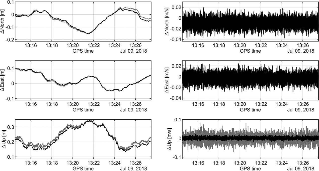
The first extended static phase took place under very good observation conditions with virtually no signal obstructions or deflections caused by the surrounding environment (see Figure 7). During the second phase, however, the observation quality was distinctly worse since the vehicle was parked south of a row of trees nearby, which resulted in higher observation noise and a lower overall number of observations. The resulting position and velocity deviations from the reference trajectory of both phases are shown in Figures 8 and 9, respectively.
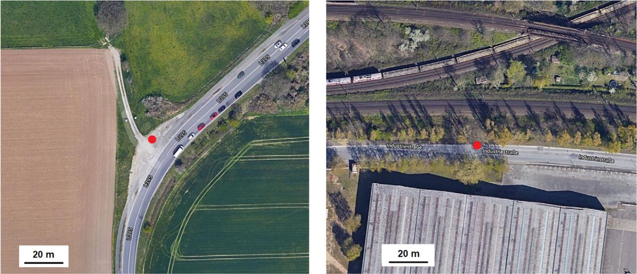
Locations where static data were recorded indicated by red dots: good observation conditions on the left, and suboptimal conditions (row of trees to the North, building to the South) on the right (map source: Google Maps)

Position (left) and velocity (right) deviations from the reference solution during the first static experiment phase with and without receiver clock modeling depicted by black and gray lines, respectively. Please mind the different y-axis scalings
Position (left) and velocity (right) deviations from the reference solution during the second static experiment phase with and without receiver clock modeling depicted by black and gray lines, respectively. Please mind the different y-axis scalings
During the first phase, the precision of the position deviations varies at the low decimeter level (i.e., roughly 15– 25 cm) where the up-coordinates also exhibit an offset of approximately 25 cm. Except for the north-component, which shows a slight offset, the velocity states scatter around zero-mean, with a peak-to-peak noise level of around 1–2 cm/s.
These values are as expected for a static PPP solution for an observation period of 13 minutes under good environmental conditions. Regarding the impact of RCM, as expected the horizontal position and velocity estimates are only slightly affected since they are not correlated with the receiver clock parameters. On the contrary, the vertical velocity estimates display an improvement of about 69% in precision and accuracy. Exhibiting a smoother shape and progression, the up-coordinates do show a precision improvement with RCM of approximately 27%, whereas their accuracy stays unchanged.
The results of the second static phase look distinctly different regarding both the magnitude and the shape of the position and velocity deviations. On the one hand, the horizontal position solutions scatter about 40–60 cm around the reference position, where, in addition, the East-component shows a mean offset of approximately −1.1 m. On the other hand, the velocity estimates exhibit a behavior similar to the first static phase, although the overall noise is increased by a factor of roughly five.
A total of 4,563 and 4,473 outliers was detected with and without RCM, respectively, as opposed to the first phase where in both solutions the exact same 37 outliers occurred. Figure 10 further shows that also the distribution of these outliers is changed when applying RCM, which leads to an observation geometry that evolves differently over time.

Number of identified and rejected outliers during the second static experiment phase with and without receiver clock modeling depicted by black and gray lines, respectively
We can also see that mainly the carrier phase observations are affected by that. In addition, with RCM the overall number and distribution of detected phase cycle slips changes slightly. As a result, each carrier phase interruption (i.e., outlier or cycle slip), causes a reinitialization of the corresponding ambiguity state parameter, hence the different positioning solutions.
For the velocity estimates, we get results similar to those of the first static phase. Although the overall noise was higher compared to the first static phase; again, precision and accuracy of the vertical component were improved by approximately 70%.
As an interim conclusion, we can state that clock modeling is very beneficial with regards to the precision of the vertical velocity estimates. The impact on the position solution is also significant, but for another reason: RCM changes the behavior of the outlier identification scheme, which ultimately leads to changes in the observation geometry.
5.1.2 Overall test drive
The position and velocity deviations from the reference trajectory of the whole experiment are shown in Figure 11. The largest differences occur in—or shortly after—situations with a very sparse and/or geometrically unfavorable observation distribution, for instance when driving through an alley or an underpass. As a consequence, the position and velocity estimates deviate up to several meters and meters per second, respectively, from the reference solution.

Position (left) and velocity (right) deviations from the reference solution of the whole experiment with and without receiver clock modeling depicted by black and gray lines, respectively. Please mind the different y-axis scalings
The formal errors of position and velocity are at the level of a few centimeters and centimeters-per-second, respectively, except for situations after an extended observation outage, for example when driving through a railway underpass. Overall the accuracy is at an expected level for a kinematic PPP solution in such an urban environment/application. In terms of RMSE, it amounts to approximately 1 m and 0.1 m/s, respectively.
When applying RCM, the clock estimates reflect the nominal behavior of the PHM and do not vary arbitrarily as much as compared to without RCM, as can be seen from Figure 12. The overall smoother courses of clock offset and drift lead to smaller position and velocity deviations. This also has an impact on the used outlier detection scheme, which will be discussed in further detail in the next subsection.
Receiver clock estimates of the whole experiment with and without receiver clock modeling depicted by black and gray lines, respectively
Overall, RCM improves the precision and accuracy of the vertical velocities by 57%. As expected, it has almost no effect on the horizontal components. For position estimates, RCM primarily reduces larger deviations from the reference solution, thus enhancing precision and accuracy by roughly 10–20%.
5.1.3 Detailed investigation
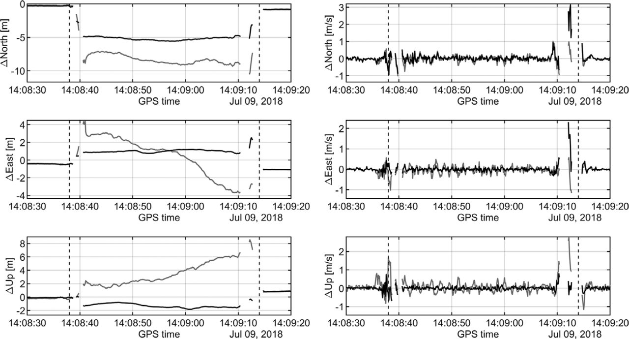
In order to illustrate the impact of RCM, we will use a specific period during the test drive around 14:09 GPS time as depicted by Figure 13, where the largest position deviations occur. Here, the vehicle was entering a North-South highway underpass from the West, stayed beneath it for approximately 30 seconds—waiting for a green traffic light—before leaving to the East. This whole sequence lasted for about 35–40 seconds. The corresponding position, velocity, and clock estimates are shown in Figures 14 and 15.
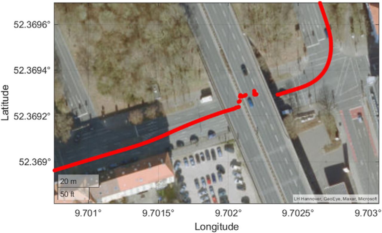
Geographical situation when driving through the underpass from the Southwest to the Northeast

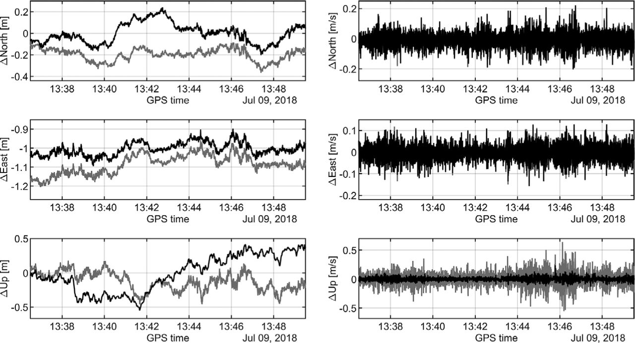
Position (left) and velocity (right) deviations from the reference solution when driving through the underpass with and without receiver clock modeling depicted by black and gray lines, respectively. Please mind the different y-axis scalings

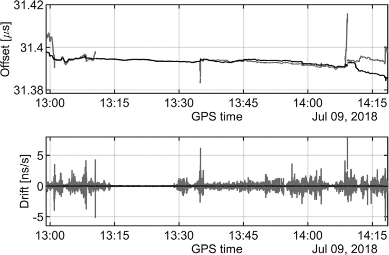
Receiver clock estimates when driving through the underpass with and without receiver clock modeling depicted by black and gray lines, respectively
The period when the vehicle was staying beneath the underpass from 14:08:37 to 14:09:14 GPS time is clearly visible in all three figures. At the start and the end of this phase, a few measurement epochs were completely rejected. During the static portion when no RCM was applied, we see stronger position deviations in all three components and more pronounced scatterings of the velocity deviations, especially in the up-component.
The reason for this can be found in the clock states depicted in Figure 15, where in the case of RCM, the estimates do not deviate from the nominal behavior of the PHM as they do when no RCM is applied. Thanks to these physically (more) meaningful clock states, the position deviations are not only significantly reduced, but also the drifts in the East- and up-coordinates are prevented. This makes sense since the spectral coefficients of the PHM do not allow such a behavior.
5.2 Reliability
The concept of reliability was introduced by Baarda (1967, 1968) and transferred to navigation by Teunissen (1990). It can be divided into internal reliability and external reliability. Internal reliability describes how large an erroneous observation has to be so that it can be detected and, as such, given a certain significance level and test quality. Typically, reliability theory is used as a planning tool since its measures can be computed without any actual observations but simply from the known observation geometry, or to be more specific, from the functional and stochastic estimation model.
In the end, internal reliability essentially determines the detectability of outliers in the observation data and is often assessed by means of the so-called minimal detectable biases (MDB). A smaller MDB means that an outlier of smaller magnitude can be assessed as such in the corresponding observation with the same probability.
One approach to determine the MDB ∇𝑙𝑖 of a single observation 𝑖 is by assessment of the cofactor matrix of the filter innovations 𝐂𝑑 and the non-centrality parameter 𝜆0:
 18
18
Transferring internal reliability values to the state domain leads to external reliability measures 𝛁𝐱𝑖, which give an indication about the impact of a single MDB on each filter state:
 19
19
where 𝛁𝐥𝑖 is an 𝑛×1-vector containing all zeros except for one MDB at index 𝑖, and 𝐊 is the Kalman gain matrix. Typically, this analysis only focuses on the position and velocity states. This enables us to derive statements about the magnitude of position and velocity deviations that can be expected.
Since a number of 𝑛 vectors is computed at each measurement epoch, typically only the maximum values are used to assess the reliability of each state. Figure 16 shows the three-dimensional maximum values of the position and velocity states at each epoch of the experiment. For better illustration, a few larger values with maximums of about 1.8 m and 14 m/s, respectively, are not depicted at this point.

External reliability during the whole experiment with and without receiver clock modeling depicted by black and gray lines, respectively
Taking the RMSE of these time series as a quality indicator, we find that RCM improves the external reliability of the position and velocity estimates by approximately 30% and 34%, respectively. This means that clock modeling makes the filter solution more robust (i.e., an undetected observation error has a smaller impact on the state estimates than without RCM). As a consequence, the overall quality of the position, velocity, and time (PVT) solution is improved.
5.3 Troposphere estimation
The troposphere state is typically highly correlated with the receiver clock offset and the vertical position states. The troposphere estimates of the whole experiment—with and without RCM—are depicted in Figure 17. Most of the time, the results are very similar and only differ by approximately 1–3 mm. However, within the last 8 minutes, both time series deviate significantly from one another.

Troposphere estimates during the whole experiment with and without receiver clock modeling depicted by black and gray lines, respectively
The maximum divergence at the very end amounts to approximately 40 mm. Due to the mentioned correlations, a similar behavior can be found in the estimates of the clock offset as well as the position, as can be seen from Figures 11 and 12. Also, as discussed in Section 5.1.2, the results with RCM make more sense since, in this case, the progression of the clock estimates is physically more meaningful than without RCM. The horizontal position states benefit from this because their estimates are much closer to the reference solution.
5.4 Carrier phase ambiguities
A critical point in PPP is the convergence time of the real-valued carrier phase ambiguities. The earlier they converge at a certain value, the earlier a specific precision level of the PVT solution is reached. In a one-way (e.g., forward processing) direction, it takes usually several minutes to achieve sub-decimeter precision of the estimated receiver position. Apart from that, in an automotive application like the one at hand, frequent signal interruptions occur which leads to a lot of reinitializations of the corresponding filter state.
Figure 18 shows two such exemplary cases for one GPS satellite (G07) and one Galileo satellite (E09). The impact of receiver clock modeling is visible as it smoothes the overall course of the state estimates. In the end, however, with and without RCM, the ambiguity state converges virtually to the same value.

Carrier phase ambiguities for satellites G07 (top) and E09 (bottom), each selected for a specific period of time, with and without receiver clock modeling depicted by black and gray lines, respectively
6 CONCLUSIONS
The use of an atomic clock—combined with an alteration of the estimation/filter model [i.e., receiver clock modeling (RCM)]—improves the overall performance of the position and velocity estimates in terms of precision and reliability. In a typical kinematic application, only an oscillator like a chip-scale atomic clock (CSAC) can be used, which restricts the PVT solution to be based on code and Doppler observations since RCM is only meaningful that way. The use of carrier phase observations requires an oscillator of at least two orders of magnitude of higher stability compared to a CSAC, for example a passive hydrogen maser (PHM).
In order to investigate the application of a PHM in a true kinematic GNSS application, we conducted an automotive experiment in the city of Hannover, Germany, on July 9, 2018. We recorded 10 Hz GPS, GLONASS, and Galileo data with a JAVAD Delta TRE-G3T receiver. For the computation of a tightly coupled GNSS/INS reference trajectory, we also recorded 200 Hz data with a tactical-grade iMAR FSAS IMU. This solution exhibits high precision for position and velocity with maximum formal standard deviations of 0.095 m and 0.014 m/s, respectively.
The kinematic PPP with and without receiver clock modeling was computed by means of the in-house Matlab GNSS software based on a forward-backward linearized Kalman filter (LKF). In the first case, the process noise model of the clock offset and drift used spectral coefficients representative for the PHM while in the case without clock modeling, the values for a typical crystal oscillator as listed in Table 2 were applied.
As a result, RCM improves the position and velocity estimates in terms of precision and accuracy by 15% and 57%, respectively. Furthermore, its reliability is enhanced by about 30%, which makes the overall solution more robust against gross observation errors.
Detailed investigations also showed that RCM prevents large position deviations in situations with a sparse and geometrically unfavorable observation geometry. Regarding the influence of RCM on other filter states like the tropospheric zenith delay and the carrier phase ambiguities, we found only small changes that have little to negligible impact on the overall PVT solution. Although the convergence behavior of the carrier phase ambiguities was altered by RCM, their convergence time was not.
With all the improvements regarding precision and reliability of position and velocity in mind, we are confident that future advancements in clock technology will make the approach of using an oscillator with a stability comparable to that of a PHM more practical for ordinary use cases in GNSS navigation.
HOW TO CITE THIS ARTICLE
Krawinkel T, Schön S. Improved high-precision GNSS navigation with a passive hydrogen maser. NAVIGATION. 2021;68:799–814. https://doi.org/10.1002/navi.444
DISCLAIMER
The authors do not attempt to recommend any of the instruments under test. It is also to be noted that the performance of the equipment presented in this paper depends on the particular environment and the individual instruments in use. Other instruments of the same type or the same manufacturer may show different behavior. The readers are, however, encouraged to test their own equipment to identify the system performance with respect to a particular application.
ACKNOWLEDGMENTS
The authors would like to thank Dr. Andreas Bauch and his team from Physikalisch-Technische Bundesanstalt, Germany, for providing the passive hydrogen maser for the kinematic experiment.
Footnotes
Funding information
Federal Ministry for Economic Affairs and Energy of Germany, Grant/Award Number: 50NA1705
Abbreviations: ADEV, Allan deviation; CSAC, chip-scale atomic clock; DIA, detection, identification, adaption; FFM, flicker frequency modulation; IGS, International GNSS Service; ISCB, inter-system code bias; MAC, miniature atomic clock; MDB, minimal detectable bias; PHM, passive hydrogen maser; PSD, power spectral density; PVT, position, velocity, time; PTB, Physikalisch-Technische Bundesanstalt; RCM, receiver clock modeling; RMSE, root-mean-square error; RWFM, random walk frequency modulation; TCXO, temperature-compensated crystal oscillator; TPE, time prediction error; WFM, white frequency modulation
- Received March 2, 2021.
- Revision received June 23, 2021.
- Accepted July 26, 2021.
- © 2021 Institute of Navigation
This is an open access article under the terms of the Creative Commons Attribution License, which permits use, distribution and reproduction in any medium, provided the original work is properly cited.


Jump to section
Related Articles
Cited By...
- No citing articles found.