Perspectives on the Systematic (Type B) Uncertainties of UTC-UTC(k)

2 THE UNCERTAINTY FORMULATION

The algorithmic definition of EAL at any epoch can be found in many places including Panfilo and Arias (2019):

2.1

where h_n is the reading of any clock at a given epoch, w_n is its weight, and is a prediction of EAL – h_n. In this expression, w_n and are based on data from previous epochs. The data consist of measured differences between clock readings, and the non-local measurements are contaminated by time-transfer noise and biases. The clock predictions in Equation (2.1) ensure some level of continuity when clocks are added or their weights are changed.

The clock predictions are based on over 50 years of data, defining the history of UTC and EAL. They are linearly related to past and present link calibration biases, and to the imprecision and inaccuracies of the astronomical data used to initialize UTC. For example, the initialization of EAL and UTC could be achieved or changed by adding a constant to all the clock predictions at the first epoch, and this would carry through to all epochs.

In the non-redundant network currently used by the BIPM, all the time-transfer links (hereafter, just links) involve a common laboratory (the pivot, whose acronym is PTB) and the link uncertainties are a mixture of station-based and link-based. Station-based data and uncertainties are properties of the station’s time-transfer equipment only. Link-based data and uncertainties are properties of the link’s time-transfer equipment instead of either station individually. GNSS data reduced via all-in-view or precise point positioning are station-based, while links involving fiber optics or two-way satellite time and frequency transfer (TW, also known as TWSTT) are typically link-based. For the purposes of this work, only GNSS data are treated as station-based. It is assumed that all measured calibration values have always been immediately incorporated into the data. The errors in those calibrations are unknown and denoted b_n if lab n’s time-transfer equipment uncertainties are station-based. The bias of the link between labs n and m is denoted b_n,m, which equals b_n – b_m if the link is station-based. Following the central limit theorem, they can be treated as stochastic quantities with normal distributions that have zero mean and standard deviations (uncertainties) σ_B,n and σ_B,n,m, respectively. If the link is based on a single GNSS observed by both labs, then b_n,m = b_n – b_m = –b_m,n and . More complex formulas are used below for cases in which two labs for UTC generation are linked via a chain of direct links involving other modes and labs.

With h_k representing any clock reading, including steered UTC realizations and devices under test (DUT), EAL at any epoch is given by

2.2

UTC minus any clock k, including a UTC(k), weighted or not, is given by

2.3

Here N_Leap is the number of the leap seconds inserted to keep UTC aligned with recent astronomical data involving Earth’s rotation, t_epoch is the time of the current epoch, and t_s is the time steer s was implemented. If leap seconds are inserted simultaneously to UTC and all clocks, they drop out of the differences and so will be ignored hereafter.

In Equation (2.3), a clock difference measurement at the current epoch is given by h_n – h_k, whereas the weights, clock predictions, and steers are functions of past data, whose detailed forms have been altered over the years. Therefore, the clock predictions can also be written

2.4

where t denotes a past epoch, tnow is the current epoch, and c_n,t defines the clock models that compute into the predictions. The last term, r_n,tREF_t, relates to the reference standard used to characterize clocks. Initially, it was solely EAL (itself a function of even more previous epochs) but currently the frequency drifts are determined using the calibrated frequency standards that define the second in the International System (SI). The c_n,t and r_n,t are often correlated across clocks and across epochs. Their functional forms are also epoch-dependent, particularly as network topologies and clock prediction algorithms have evolved. The weights, w_n, and EAL-steering terms, y_s, are functions of past measurements, but they are based on inferred frequencies and are thus independent of the time-transfer biases. Since they do depend to some extent on the statistical errors in measurements of previous epochs, ignoring them in computing Type A uncertainties of UTC-UTC(k) is a decision rather than a requirement.

Equation (2.4) is unwieldy and included merely to clarify the idea that the uncertainty of UTC-UTC(k) depends on which unknown biases and epochs one wishes to consider as contributing to the uncertainty of UTC-UTC(k), and which to consider as having no uncertainty contribution. Terms without uncertainty are considered to have become part of the numerical definition of UTC, which, once published, is never recomputed. Returning to Equation (2.3), the law of propagation of uncertainties (JCGM/WG 1, 2008) relates the overall uncertainty to the bias and noise derivatives of Equation (2.3) that one considers applicable. For systematic uncertainties, a variation, δ, due to an unknown bias is equivalent to the derivative with respect to that bias variable being multiplied by the bias value itself, and can be applied to Equation (2.3) as:

2.5

Since the algorithm computes steers and weights based on frequency measurements, which have no bias contamination, the last summation of Equation (2.5) can be ignored, resulting in

2.6

2.7

In Equation (2.7), the first summation embodies the measurement data of the epoch in question, and the second summation is corrupted by the systematic uncertainties of the initialization and past measurements. Note also that all clocks measured at a given institution bear identical variations and uncertainties with regard to UTC. Among other reasons, this is because their local measurements are assumed to have negligible bias and noise. Therefore, for brevity, it will hereafter be assumed that every lab has one clock and that this clock, though unsteered, serves as the lab’s UTC realization.

In the instantaneous approach, currently used by the BIPM, none of the derivatives from past epochs are retained and the second summation in Equation (2.7) is ignored. It was noted in M2020 that the resulting uncertainties in UTC-UTC(k) represent the statistics that observers who had installed extremely high-quality optical fibers between the labs would find when using their data at the epoch in question in concert with the pre-determined weights and clock predictions. This approach has been criticized because it has no use for the correlations between the biases of previous epochs and clock predictions (G. Petit and G. Panfilo, personal communication, November 14, 2020). The bias correlations between epochs are not relevant in this approach because the predictions for the current epoch are predetermined and, on this basis, considered an immutable and numerical part of the definition of UTC.

To the opposite extreme, one might wish to consider every uncertainty indicated by Equations (2.3) and (2.4). Unfortunately, the uncertainties of the astronomical data in the early 1970s were of order 1.5–2 ms (D. McCarthy, personal communication, March 28, 2022) and the time transfer uncertainties in the 20th century started at the microsecond level (Guinot et al., 1971) while falling to a 10-ns level later. They are now at the several nanosecond level. The systematic uncertainty of UTC-UTC(k) would grow without limit as each new link calibration adds its contribution to the older ones.

A good compromise between the historical and instantaneous approaches would be to consider, for each extant link only, the bias dependencies of the epochs since the last calibration. As with the instantaneous approach the effect of no-longer used calibrations and the astronomical initializations, embodied in the clock predictions, are ignored. These can be considered hardwired or calcified parts of a frequently-redefined definition of UTC. This will be termed the semi-historical way hereafter. It follows the philosophy, though not the letter, of PPH2020, and this paper is dedicated to exploring its consequences.

3 A PIVOTLESS SINGLE-GNSS NETWORK IN THE SEMI-HISTORICAL APPROACH

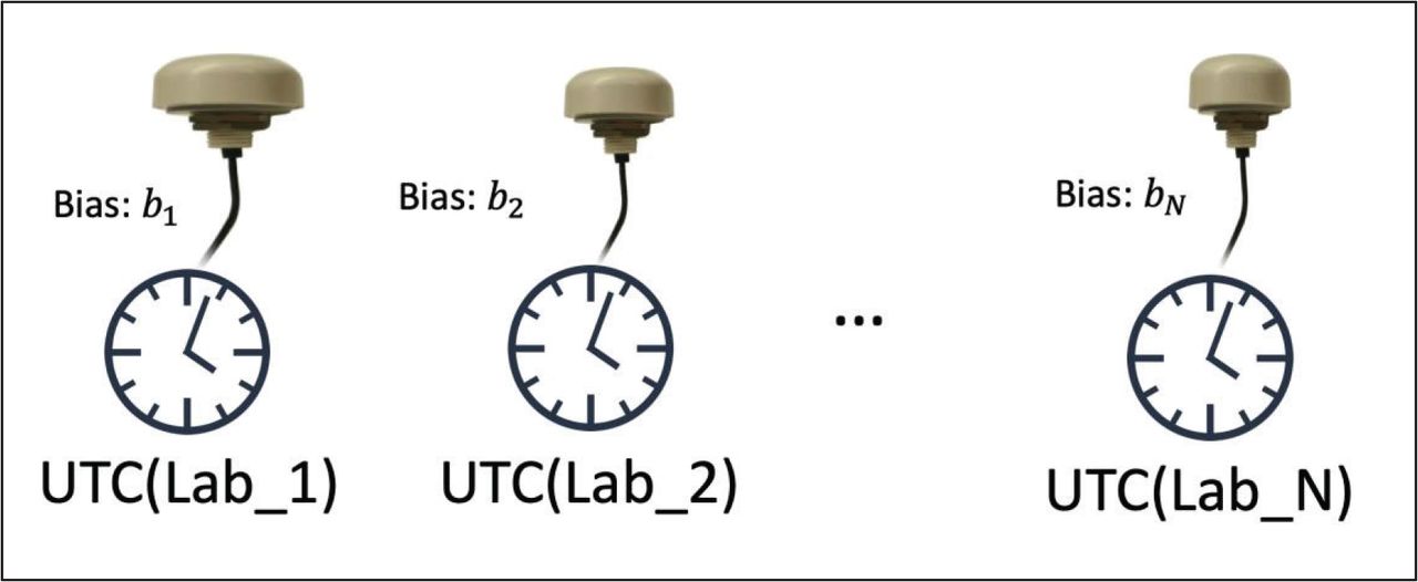
A network utilizing a single GNSS system has no pivot lab (Figure 1), and all the uncertainties are station-based. In this section, it is shown that the biases in UTC-UTC(k) may initially have a range of values, but in the semi-historical approach they will evolve towards a simple result in which each lab’s uncertainty with respect to UTC exactly equals that of its own GNSS system’s calibration. That evolution will include new labs being incorporated into UTC, and be complete once every initial lab has had its GNSS setup recalibrated.

• Download figure
• Open in new tab
• Download powerpoint

FIGURE 1

A single-GNSS network has no pivot to the extent the uncertainties are station-based.

A formula that explicitly shows the (unknown) biases of a station-based measured clock reading is:

3.1

where h_n0 is the true clock reading, which would be observed in the difference with other clock readings if there were no biases in the measurements. If a second GNSS system is involved (such as Galileo), the subscript S may be included for clarity, such as b_nS.

The difference between the station-based clock readings of labs n and m, can be written

3.2

The bias contamination of Equation (2.7) is

3.3

Since the weights are normalized

3.4

In the instantaneous approach, only the uncertainties of measurements at the epoch in question are considered. The clock predictions are considered immutable, and the second summation becomes zero.

3.5

The statistics are given by the square root of the average value of the square of the right-hand side. In this case, since the noise and biases are uncorrelated, the squared systematic and statistical uncertainties are given by

3.6

Identical formulas can also be derived for Type A uncertainties, based on the noise rather than the biases. Since past history is intentionally ignored, the statistics can be computed via least-squares solutions that use just the measurements and uncertainties of the extant links. Lewandowski et al. (2006, 2008) presented a means to mathematically compute the above expressions for both station-based and link-based uncertainties, and equivalent matrix formulations were given in Matsakis (2020, 2021).

If one wishes to include the uncertainties associated with past data, it is possible to derive a very plausible solution that utilizes the fact that systematic errors are systematic. It requires the assumption of PPH2020 that the clock predictions are linearly related to the bias of only their own lab’s time-transfer equipment as follows:

3.7

where is what the clock prediction would be if lab n’s GNSS system’s unknown bias were exactly zero, as it is assumed to be in UTC computations. This relation is plausible because the BIPM creates predictions for a new lab based upon a period of observations in which the laboratory had no weight in UTC. Inserting this relation into Equation (3.4) yields

3.8

Since the bias terms in the summation have been eliminated, the square root of the average square immediately yields

3.9

where σ_B,k is the uncertainty of the GNSS equipment at lab k, and h_k can be UTC(k) or any clock locally measured against UTC(k) and, as noted, this result depends upon the validity of Equation (3.7).

However, the premise only applies if the initialization biases can be ignored. Assuming the network was initialized by independently measuring each lab’s clock against an external standard the initial predictions would be given by

3.10

where b_n,initial is the bias related only to the initialization at the first epoch. Once initialized, links with biases b_n are placed into use, but their biases would not be cancelled inside the summations that define EAL/TAI/UTC. Without this cancellation, the analog to Equation (3.8) becomes

3.11

If one is willing to ignore the millisecond-level initialization biases when the initialization is via astronomical means, this formula is identical to Equation (3.5), and leads to the uncertainties as computed by the instantaneous approach. That formula would also be recovered if the initialization was by means of a simple bootstrap in which each clock’s reading was taken as is, for then b_n,initial = 0 at the start. In another variant of this approach, let the first lab’s initial clock reading be the initialization standard. Then b_n,initial = b_n – b₁, and so the unknown bias and therefore the uncertainty of the first lab’s GNSS calibration contributes to that of all other labs. A similar result happens if the first lab was initially the only lab, and the other labs were subsequently added—mathematical derivations of these are given in the next section.

As new labs are added, the unknown initial biases will corrupt the predictions for them. This is because those biases will contaminate the observations used to establish the predictions for the new labs. The uncertainties of these labs would be the square root of the average value of the square of Equation (3.5), except that the summation would only include the original N labs, whose weights would no longer sum to 1. Note that the converse is not true. Biases of the new labs will not affect the predictions or uncertainties of the original N labs because the bias corruption of the new labs’ clock predictions will nullify the biases of the measurements involving their clocks.

Although the semi-historical approach does not yield the simple result of Equation (3.9) at initialization, it will approach it as the original labs recalibrate or upgrade their GNSS setups. The change is mathematically equivalent to completely downweighting the recalibrated lab and introducing a new lab that just happens to have the same clocks. As with the labs added after initialization, its clock predictions are revised so as not to impact UTC. Assume for definiteness that it is Lab N, its GNSS system’s uncertainty b_N is replaced by the new uncertainty b_{N, new}, and its clock model is adjusted by b_N – b_{N, new} according to the findings of the recalibration. Since b_N no longer describes an extant link, its contribution to the uncertainty of all the other labs is ignored and there is one less lab contributing to the summations of Equations (3.3), (3.8), and (3.11). Since the initialization biases are ignored, Lab N then has a bias contamination equal to . Once every lab in this pivotless network has been recalibrated there are no terms left in the summation, and the bias contamination of each lab is just that of its own time-transfer system. The uncertainty of every UTC-UTC(k) then equals the uncertainty of Lab k’s GNSS system, and Equation (3.9) is fully valid.

This does not mean that the actual value of each UTC-UTC(k) is independent of what the initial biases were; only the dependence of each UTC-UTC(k) on the calcified biases and their contributions to the clock predictions is ignored. For those labs that steer their clocks so that UTC-UTC(k) is near zero, it is the amount of steering applied by the labs that would be dependent on the past biases.

4 PIVOTS WHEN ONLY EXTANT LINKS ARE CONSIDERED (SEMI-HISTORICAL)

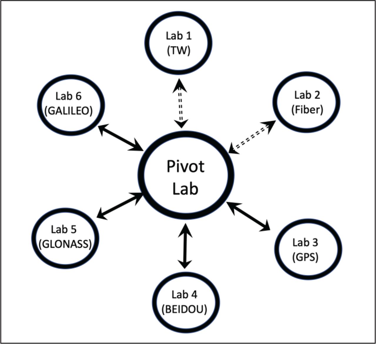
The network used to compute UTC has evolved over the years, and will continue to do so. Figure 2 shows multiple link types, although UTC is currently computed with TW, fiber, and GPS links connected to the pivot lab. In the future, modes may be used in parallel, and crosslinks directly used.

• Download figure
• Open in new tab
• Download powerpoint

FIGURE 2

The topology of a single-pivot multi-mode non-redundant network. Links with station-based uncertainties are identified with a single solid arrow; those with link-based uncertainties are shown with dashed double-arrows.

Pivots are inevitable when more than one time-transfer mode is used because the definition of EAL requires every clock to be differenced with every other one. For a measurement involving labs with dissimilar modes, differencing the labs requires differencing through a chain of labs including at least one pivot lab for which both modes are enabled. For a GNSS-enabled lab, n, and a TW-enabled lab, m:

4.1

where p refers to a pivot lab. If the measurements in Equation (4.1) are station-based and of the same mode, their bias contamination is

4.2

If the measurements are link-based, all that can be written is:

4.3

And if the modes at the pivot are different but both station-based, such as GPS and Galileo,

4.4

where b_pS refers to the bias of the pivot’s second station-based system, S.

Consider how one can build up a network from one lab to two labs and then to the three labs shown in Figure 3. With no loss of generality, we can assume that each lab has only one clock whose unsteered output is its UTC realization, no leap seconds are inserted, and there is no steering of EAL, so that UTC=TAI=EAL. The semi-historical approach ignores initialization uncertainties, but we can alternately assume that any initialization constraint of interest has been incorporated into the first lab’s clock reading or clock predictions with negligible uncertainty. While for simplicity only one lab is added at a time, the generalization to many initial labs and many simultaneous new lab additions is straightforward.

• Download figure
• Open in new tab
• Download powerpoint

FIGURE 3

Lab #1 is the sole lab until Lab #2 is linked to it by GPS. Later, Lab #2 becomes a pivot linked to Lab #3 via a second station-based mode as shown, or by TW.

When there is just one lab, the UTC timescale originally is just the output of that one lab’s clock, adjusted by an ignorable initialization constant. The calibration status of any time-transfer equipment at this point is irrelevant for UTC, although it would be important for any user attempting to access that lab’s UTC realization non-locally. The bias contamination of any predictions for that lab’s clock(s) would be zero, and so would be the uncertainties in UTC-UTC(k=1).

When a second laboratory is added, its introduction is required to have been preceded by an extended period when the second lab’s clock was observed against UTC as defined by the first lab. During this period the data for the first lab has no bias contamination, as the second lab’s clock is unweighted, so that

4.5

Whether the link is via TW or GNSS, the bias-contaminated difference between the clock readings of the new lab and the lab that is still defining UTC would be:

4.6

From Equation (4.6), the observation period for the second lab will result in the predictions

4.7

Thus the full uncertainty of the link is incorporated into the predictions for the new lab, including the contribution from the first lab’s GNSS system if the link is station-based. Once the second laboratory is weighted, Equation (2.2) yields

4.8

where hereafter prediction terms will be identified by being enclosed in brackets where they are first used.

4.9

So the bias contamination to UTC – h₁ remains 0 (for any time-transfer mode). In other words:

4.10

Using the clock predictions of Equation (4.3), the newly weighted lab’s difference with UTC is given by:

4.11

4.12

4.13

The bias contamination of UTC – h₂ is therefore –b_2.1, which, if the link is station-based, can be decomposed into b₁ – b₂.

Following the standard statistical reasoning used throughout this paper, the uncertainty of the two labs would be a special case of Equation (3.9)

4.14

4.15

where, for a GNSS link with station-based uncertainties, .

If the second lab had been the initial lab, the uncertainties would be reversed, and this shows that it is not always possible to determine the systematic uncertainties in UTC-UTC(k) using only the measurements, weights, and uncertainties of the epoch in question. However, if the first lab’s GNSS system were recalibrated,the second lab’s prediction would be adjusted by the difference between the old and new calibrations. Following the semi-historical approach, the corruption from the old calibration of the first lab would be ignored for the purpose of computing the uncertainties. The bias corruption of the new lab would be considered to be only that of its newly recalibrated system so that Equation (3.9), U_B,UTC–hk = σ_B,k, would apply fully and without reservation. It can be shown that, if other labs had been added pre-recalibration, their uncertainties would be corrupted as was the second lab’s. Once all the initial labs had been recalibrated, the fully mature network would again be described by Equation (3.9).

Assume now that the first lab has been recalibrated and the bias corruptions of the predictions of each GNSS lab, k, have become b_k. When a new lab linked by a different mode is added, a period of unweighted observations is again used to generate its clock predictions. For simplicity, we assume the new lab is the third, as in Figure 3. In this configuration, the second lab is now the pivot lab (designated p) so that a measurement of h₁ – h₃ is achieved by double-differencing with the pivot:

4.16

4.17

During the evaluation period, the contribution of biases to the first two labs’ predictions remain b₁ and b₂, and the data from the third lab yield:

4.18

4.19

If the third lab is linked to the pivot via TW, then b_p,3 is the unknown bias of the TW system. If the third lab is linked via different GNSS from the first two labs, denoted S for station-based, then b_p,3 = b_pS – b₃ and the uncertainty of that link is the root-sum-square (RSS) of the uncertainties of the two relevant other GNSS systems. Either way once the third lab is weighted the bias contribution to its difference with EAL will be:

4.20

4.21

If the first lab had not been recalibrated before the third was added, the above equation would have an additional term, . Either way the uncertainties of the first lab and the pivot would be that of their own GPS system at most, whereas the third lab’s uncertainty would depend on at least the pivot lab’s calibration uncertainty as well. While in this section only three labs have been considered, it is straightforward to show that in a mature single-pivot topology whose earlier links were GPS-only,

4.22

4.23

4.24

Note that the only thing to distinguish the GNSS systems is which one was used first. The next section will show that these same formulas apply when the pivot lab’s GPS system is recalibrated, provided the predictions for the pivot as well as all labs linked to it by non-GPS modes are adjusted accordingly.

5 RECALIBRATING PIVOTS AND THE SEMI-HISTORICAL APPROACH

The previous section showed that it is important to know what links to a pivot were established first. This section uses that information to develop a scenario in which a mature (every system recalibrated) pivotless GPS-based system is augmented with new labs linked by TW and a non-GPS station-based system (S), utilizing a common pivot lab, p. Equation (2.2) can be rewritten with separate summations for the GPS, TW, pivot, and S-linked labs as follows:

5.1

where the pivot lab, p, is excluded from the summations and the semicolon indicates that only the described terms are included in them. Following the reasoning of the previous section, if every lab except the pivot had been recalibrated the contaminations of the clock n’s predictions before recalibration are given by −b_n if it is a GPS-linked lab including the pivot, −b_p – b_p,n if it is a TW lab, and −b_p + b_pS – b_n if it is a lab linked to the pivot by a second station-based mode. Inserting these predictions within the brackets:

5.2

Before the pivot’s GPS calibration is adjusted the bias contaminations within the first summation are all only −b_k and so for any GPS-linked lab including the pivot

5.3

where and it is noted that if k is a pivot lab, some b_k terms simply cancel their neighboring b_p terms.

5.4

After a recalibration of the pivot’s GPS system, the pivot’s clock predictions will be adjusted for the difference in calibration values, and the associated unknown GPS bias will be b_pnew. It is important that the predictions of the TW-linked and S-linked labs also be adjusted. In this case, the bias contamination of the post-calibration equation remains as in Equation (5.4), where b_p only appears if k is the pivot, in which case it is now b_pnew.

Note that if the predictions of the TW and S-linked labs had not been adjusted, the bias contamination of their predictions would still be b_p, and the formula would have been

5.5

where and . The uncertainties of UTC minus the non-GPS labs would also yield weight-dependent results if the clock predictions of the labs downstream for the GPS labs were not adjusted to compensate for the pivot lab’s recalibration.

From Equation (5.2), the pre-recalibration bias contamination of the TW-linked lab would be:

5.6

If the clock predictions for all TW-linked and S-links labs are adjusted by replacing b_p with b_pnew, the post-recalibration contamination is

5.7

From Equation (5.2) the pre-recalibration bias contamination of a lab linked by station-based system S would be:

5.8

5.9

Therefore, for every lab in the network, the only change in the bias contamination of EAL – h_k is that b_pnew replaces b_p in the formulas. The variations of the links can be converted into the uncertainties of UTC-UTC(k) as follows:

5.10

5.11

5.12

HOW TO CITE THIS ARTICLE

Matsakis, D. (2023). Perspectives on the systematic (Type B) uncertainties of UTC-UTC(k). NAVIGATION, 70(2). https://doi.org/10.33012/navi.571