

Abstract
The success of future lunar missions depends on quality positioning, navigation, and timing (PNT) information. Earthbound GNSS signals can be received at lunar distances but suffer from poor geometric dilution of precision (GDOP) and provide no coverage of the lunar far side. This article explores the design space of a dedicated GNSS system in lunar orbit by using a multi-objective evolutionary algorithm framework to optimize GDOP, availability, space segment cost, station-keeping ΔV, and robustness to single-satellite failure. Results show that Pareto approximate solutions that achieve a global GDOP availability (GDOP ≤ 6.0) greater than 98% contain a minimum of 24 satellites in near-circular polar orbits at an altitude of ~2 lunar radii. The impact of single-satellite failure on GDOP outage is analyzed and a no-maneuver scenario is considered. Design rules characterizing optimal solutions are identified and trade-offs between station-keeping maneuver frequency, performance, and design lifetime are discussed.
1 INTRODUCTION
Recent direct and definitive evidence of surface-exposed water ice in the lunar polar regions (Li et al., 2018) has changed our perception of the Moon. The identification of these resource-rich locations has transformed the economics of Moon mining (Sommariva et al., 2020) and established Earth’s satellite as an interesting destination for the private space sector. As a consequence, this decade has seen a plethora of planned lunar missions and the establishment of new public-private partnerships.
This article analyzes the case for a lunar GNSS by exploring the design space in a high-fidelity lunar environment and evaluating design trade-offs in terms of performance, cost, and robustness objectives. The investment in a dedicated GNSS in lunar orbit can be justified by the need to execute complex maneuvers—rendezvous, docking, and precise landing—that depend on the supporting positioning, navigation, and timing (PNT) infrastructure.
According to the International Space Exploration Coordination Group (ISECG) Global Exploration Roadmap (ISECG Technology Working Group, 2019) the future mission PNT performance targets are: a) absolute and relative position accuracy of less than 0.4 m; b) timekeeping accuracy down to nanosecond level; and c) inter-element time synchronization without dependence on Earth-based systems.
These targets are beyond what can be achieved with present autonomous deep-space navigation systems (e.g., simulations using optical navigation measurements and JPL’s AutoNAV filter show that lunar landings are only possible to within 20 m [Riedel et al., 2010]). Thus, current deep-space missions rely on Earth-based communication links (e.g., via two-way Doppler and range or delta-differential one-way range). Yet, the Deep Space Network (DSN) is operating close to capacity (Abraham et al., 2018), which poses concerns in terms of availability of service for future missions.
This level of absolute navigation accuracy (< 0.4 m) can currently be met in low Earth orbit (LEO) using dual-frequency pseudorange and carrier-phase GNSS observations even without external augmentation data, thanks to precise GNSS broadcast ephemerides as reported in Hauschild and Montenbruck (2021). Relative navigation in LEO at millimeter levels can be achieved using GPS carrier phase measurements with fixed integer ambiguities, as demonstrated in recent formation flying missions such as GRACE and TanDEM-X (Allende-Alba & Montenbruck, 2016).
1.1 Weak GNSS Signal Tracking
One approach to improve the PNT performance in cis-lunar space is to track weak Earth GNSS signals as studied in Capuano et al. (2015), Impresario et al. (2018), and Palmerini et al. (2009). This approach relies on the exploitation of antenna main lobe overspill and sidelobe tracking. Recent results from the Magnetospheric Multiscale Mission (MMS) show that a high-sensitivity GPS receiver (~23dB-Hz acquisition/tracking threshold) equipped with a 7-dB gain antenna can track the L1 C/A code of one GPS satellite on average at half the Earth-lunar distance (Parker et al., 2019).
Informed by these results, simulations show that it is possible to acquire GPS signals as far away as the moon using an antenna with a peak gain of 14 dB (Winternitz et al., 2019). Besides, it is reasonable to expect significant performance improvements from the adoption of the United Nations’ International Committee on GNSS Recommendations (United Nations, 2018). These recommendations include support for an interoperable multi-GNSS space service volume and the development of interoperable multi-frequency space-borne GNSS receivers.
This approach suffers from two limitations. First, geometric diversity (i.e., dilution of precision [DOP]) would be poor at lunar distance. Simulations of the Deep Space Gateway’s Near Rectilinear Halo Orbit (NRHO) about the Moon show that the position dilution of precision (considering GPS, GLONASS, GALILEO, and BeiDou) is greater than 250 (Delépaut et al., 2020). Thus, the problems that geometry poses limits the achievable accuracy.
The use of an onboard navigation filter and an atomic clock has effectively been able to decorrelate clock from range errors (Lopes et al., 2014). Yet, simulation results of an uncrewed mission to the Gateway NRHO considering an extended Kalman filter and a rubidium atomic clock show that the GPS-based navigation error is approximately 8.5 m (3-RMS) radially and 30 m (RSS) laterally (Winternitz et al., 2019). These figures are still far from the performance requirements identified before for cislunar navigation.
Second, there would be no coverage on the far side of the Moon. Though largely unexplored, this region contains the Aitken basin, which is one of the most scientifically interesting impact craters and a target for future missions (Kring & Durda, 2014).
Given these limitations, Earth GNSS signals are likely to be used mainly in support of orbit determination and time synchronization operations in lunar orbit, hence our focus on a dedicated GNSS in lunar orbit.
1.2 Challenges in Lunar GNSS Design
The problem of designing a stable GNSS constellation in lunar orbit is challenging due to third-body perturbations caused by the Earth’s gravitational field. This type of perturbation is dominant at orbit altitudes greater than 1,500 km (Nie & Gurfil, 2018), which is a reasonable target for a global GNSS constellation (a satellite at 1,500 km will cover no more than 19% of the lunar surface assuming an elevation cut-off angle of 5 degrees).
Orbital perturbations require station-keeping maneuvers which can become prohibitive in terms of ΔV and propellant requirements. It is generally desirable that the magnitude and frequency of station-keeping maneuvers be minimized. A low frequency of maneuvers would improve satellite availability (assuming the satellites are declared unhealthy during burn executions as it is done today with GPS) and keep operational costs down—especially if communication with Earth stations is necessary.
Savings in propellant fuel also cause reduced satellite mass and launch costs. On the other hand, a higher frequency of maneuvers could potentially improve GDOP performance, which motivates further exploration of these trades. This design problem has conflicting performance objectives that must capture performance in a complex dynamic environment, making it well-suited to the use of multi-objective optimization algorithms, since they eliminate the need for subjective preference elicitation.
1.3 Literature Review
The design space of a GDOP-optimizing GNSS constellation in a high-fidelity lunar environment remains largely unexplored, given the high computational costs involved. There have been few studies considering the design of lunar navigation satellite constellations, and the analysis has been limited to a small number of pre-defined constellations based on expert intuition. For example, Sands et al. (2006) used a generalized GDOP formulation to study the performance—in terms of the latency to achieve a performance target when integrating range and range-rate measurements—of seven sparse constellations with less than 12 satellites each.
The results highlight the improvements in performance brought by augmentations such as user altitude knowledge and highly stable user clocks. Ely and Lieb (2006) presented designs for satellite constellations in a linked-chain configuration that could achieve global coverage over a period of 10 years without station-keeping maneuvers. However, these constellations were not able to achieve global coverage with GDOP values of six or less—which are characteristic of Earth’s GNSS and would allow instantaneous 3D positioning and timing services.
Finally, there are ongoing initiatives that attempt to address stakeholder needs for PNT, networking, and scientific services (LunaNet [Israel & Mauldin, 2020]) using a combination of small satellites, lunar surface beacons, and existing GNSS signals, but to the best of our knowledge, no studies resulting from these initiatives have been published yet.
The studies mentioned above are based on the evaluation of a few expert-selected constellations. There are many constellation design studies based on optimization but none for a lunar GNSS. Finally, we note the prevalence of evolutionary algorithms in the constellation design literature (Buzzi et al., 2019; Ferringer et al., 2007; Ferringer & Spencer, 2006; Singh et al., 2020; Whittecar & Ferringer, 2014).
1.4 Research Objective
In a preliminary study (Pereira & Selva, 2020), we analyzed the performance of lunar GNSS constellations obeying frozen orbit conditions (including J2, C22, and third-body perturbations), existing when the argument of periapsis (ω) equals 90° or 270°—assuming the Earth was in a circular equatorial orbit around the Moon. It was found that the optimal constellations resulted in poor performance at the poles, which was undesirable given that many future missions have been targeting these resource-rich regions. This article greatly expands the scope of the preliminary study by re-formulating the problem (allowing for hybrid constellations mixing satellites at various altitudes and inclinations), and removing the frozen orbit constraints. Thus, it explores a much larger portion of the design space than previously done in the literature.
More specifically, this study attempts to find lunar GNSS constellation designs that minimize GDOP on the lunar surface, maximize GDOP availability (percentage of time where GDOP < 6.0, a typical mask value in DOP analysis), minimize space segment cost, minimize station-keeping ΔV, and maximize robustness to single-satellite failure. The GDOP, cost, and robustness objectives are often considered in GNSS constellation design. The station-keeping ΔV objective is justified given the magnitude of third-body perturbations in lunar orbit and the need to identify ΔV-efficient, as well as operationally feasible, designs.
Variance-based sensitivity analysis is conducted for every design decision and objective metric to capture first-order effects and important design variable interactions. Finally, we identify design rules that characterize common features of optimal solutions and analyze the main design trade-offs. In particular, in the context of a no-maneuver scenario, we investigated if the lack of a propulsion system could lead to mass and cost savings.
The rest of this article has the following structure. Section 2 describes the methodological approach and algorithms used to explore the design space of the problem and interpret the results. First, the complete multi-objective optimization formulation is introduced with a brief discussion on how the design space is constrained based on the underlying assumptions. Second, the performance, cost, and robustness metrics are derived. Third, the Multi-Objective Evolutionary Algorithm framework (Borg MOEA [Hadka & Reed, 2013]) is succinctly described along with its parameterization and indicator for search performance. Finally, the approach to sensitivity analysis and design rule mining is discussed. Section 3 presents and examines the results obtained in scenarios with and without station-keeping maneuvers. Section 4 reports the results from the sensitivity analysis and rule mining studies. Finally, Section 5 provides the conclusions, limitations, and suggestions for future work.
2 METHODS
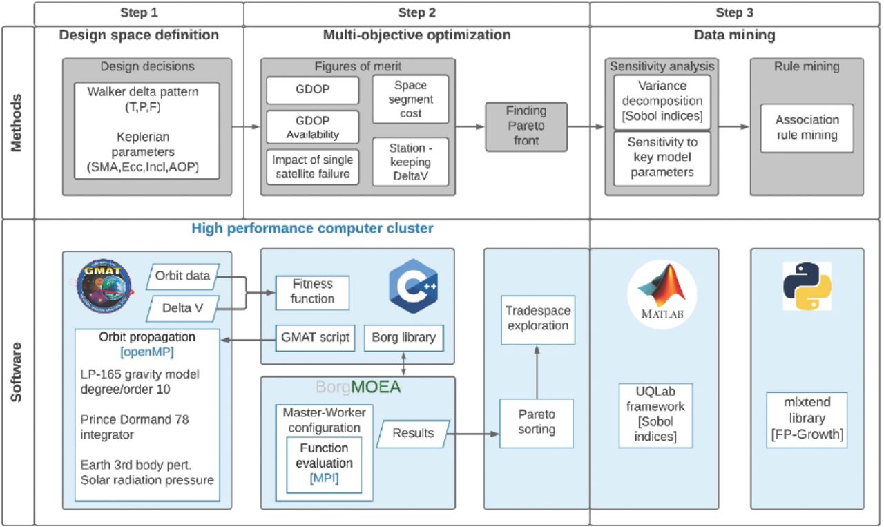
The research method used in this article is shown in Figure 1. First, the problem formulation is introduced by defining the design decisions and their range of validity. Second, the multi-objective optimization algorithm evaluates and ranks each design in terms of five figures of merit.

Research methods and software setup
In particular, Borg MOEA is used to explore the objective space based on the inputs from high-fidelity orbit simulations—done in NASA’s General Mission Analysis Toolbox (GMAT [NASA, 2019]). This software setup runs in a high-performance computer cluster with hybrid parallelization (OpenMP and Message Passing Interface [MPI]). Finally, we map the sensitivity of results to design decisions and key model parameters and identify frequent data patterns in the form of design rules.
2.1 Problem Formulation
Informed by the results obtained in our previous work (Pereira & Selva, 2020), we adopted a more general problem formulation that allowed for the consideration of hybrid constellations. In this study, hybrid constellations are assumed to consist of two different Walker constellations, which allowed for an interesting mix of orbital patterns (e.g., polar and equatorial orbits).
To have a manageable number of design variables and reduce the size of the design space, the following conditions are imposed: First, the argument of periapsis (ω) is restricted to 90 or 270 degrees. This choice of values allows the consideration of frozen orbits existing at a wide range of orbit altitudes (as long as the periapsis altitude is greater than the Moon radius); frozen orbits conditions at ω = 0°, 180° exist only up to a maximum altitude of ~1,600 km (Nie & Gurfil, 2018). Second, the number of planes (P) must be a factor of the number of satellites (T). Third, satellites in the same orbital plane are equally spaced in that plane. Fourth, the relative phasing of satellites in adjacent orbital planes (F) can only take integer values between 0 and P-1 as defined in a Walker delta pattern (Walker, 1977).
The design space is defined by a combined 14 continuous and discrete variables as shown in Table 1. Borg MOEA is configured to return real design variables in the 0–1 range. The continuous variables are scaled according to the range of values shown in Table 1. The continuous-to-discrete conversion is shown in Table 2.
Architecture Design Decisions
Continuous-to-Discrete Variable Conversion
The range of semi-major axis values is between two and 10 times the mean lunar radius (1,737 km), which seems reasonable given that existing GNSSs are characterized by nearly circular orbits at an altitude of ~3 Earth radii. The range of eccentricity values is in the interval [0–0.7] to allow for the consideration of frozen elliptical inclined lunar orbits (Ely, 2005). The number of satellites of the second constellation (variable T2) could be used to define hybrid constellations (T2 > 0), Walker constellations with more than 30 satellites (T2 > 0 & X = X2, where X represents any of the orbit parameters [SMA, P, F, e, i, ω]), and Walker constellations with up to 30 satellites (T2 = 0), in which case only the first seven variables would be considered for evaluation. At every generation, the offspring generated by Borg MOEA is evaluated in terms of five objectives, as described in the Section 2.2.
To best appreciate the importance of station-keeping maneuvers in the overall performance, we considered a station-keeping maneuvers scenario (Scenario I) and a no-station-keeping maneuvers scenario (Scenario II).
In scenario II, the station-keeping ΔV and robustness metrics were replaced by a minimizing objective metric: GDOP degradation. This metric was computed as the absolute slope of the linear least-squares fit on the monthly GDOP values (98th percentile) obtained over five years. This linear regression was sufficient to capture the overall GDOP trend.
Finally, in Scenario I, we analyzed the impact of weak GNSS signal tracking from Earth on GDOP levels at the lunar surface. Earth GNSS signals have proven desirable not only for improving GDOP but also for time transfer and synchronization of Earth and lunar GNSS time references.
2.2 Figures of Merit
Five figures of merit or metrics are used as objectives in the multi-objective optimization, including three performance metrics (GDOP, GDOP availability, and station-keeping ΔV), space segment cost, and robustness to single-satellite failure.
2.2.1 Performance
The performance metrics used in this study require detailed knowledge of satellite orbit position around the Moon over a long period of time. Thus, a high-fidelity orbit propagation software (GMAT) was used to define the inertial lunar frame, propagate the satellite orbits, and implement the station-keeping maneuver strategy. The adaptive step Prince Dormand 78 integrator (eighth order Runge-Kutta) was used to propagate the orbits under the following force model: a) Lunar LP-165-P gravity field model with spherical harmonics up to degree and order 10; b) Earth’s third-body perturbations; and c) solar radiation pressure using the default spherical shape and reflectivity. The orbits were defined in an inertial frame centered at the Moon and referenced to the lunar equator at the J2000 epoch. The orientation of the Moon was defined by Euler angles given in the DE-421 JPL planetary ephemeris.
GDOP
GDOP is used to provide a measure of satellite geometric diversity on the lunar surface. GDOP is important because this geometry factor is multiplied by the user equivalent range error (UERE) to produce an estimate of the user 3D position/time solution. Thus, we sought satellite constellations that could consistently produce low GDOP values. In this article, we make no assumptions in terms of the UERE, but the error budget is likely to be driven by satellite clock and ephemerides errors, especially if ground and control segment operations are made solely from Earth.
The range error component due to the Moon’s ionosphere is expected to be small but not negligible (Stubbs et al., 2011). Investigations from Luna 19 and 22 spacecraft radio occultation measurements indicated that a high concentration of electrons could result from photoemission and secondary emission from exospheric dust (Stubbs et al., 2011). The same study showed that despite its highly variable nature, these electron concentrations could be ~103 cm−3 at altitudes of up to 10 km, which is similar to the values present in Earth’s Ionospheric D region.
In this study, GDOP was computed assuming a 5° elevation angle and a user grid formed by 500 equidistant points on a sphere with radius equal to 1,737 km (mean lunar radius). Despite the effort to correct for orbit perturbations, GDOP degradation over time is to be expected if station-keeping maneuvers prove to be ineffective. Therefore, the GDOP was computed at 480 points in time (obtained with Latin Hypercube Sampling [LHS]) over one year—long enough to capture the eventual GDOP degradation.
The GDOP metric is defined as the 98th percentile of all GDOP samples (in space and time) with a value less than six. This metric is particularly useful in identifying the designs with the best geometric diversity among the global constellations (GDOP availability ≅ 100%). The C++ implementation used a closed-form equation for GDOP computation that used less operation counts than a typical LU matrix inversion (Doong, 2009). Finally, orbit designs that would have led to satellite collision with the lunar surface or to satellites escaping the lunar’s sphere of influence were penalized with a GDOP equal to 10.
GDOP Availability
The GDOP availability metric is an indication of the systems’ ability to provide usable service as defined by a minimum acceptable target value (GDOP = 6.0). This metric is used to identify global designs, which are characterized by a GDOP availability ≅ 100% and thus can achieve GDOP ≤ 6 at any time and location on the lunar surface. The GDOP availability metric was computed as the percentage of GDOP samples—out of a total of 240,000 GDOP samples generated (500 grid locations at 480 points in time)—with a value equal or less than six.
Station-Keeping ΔV
This metric provides an indication of the operational feasibility of different orbit designs. Station-keeping ΔV magnitudes were computed analytically using equations from Schaub and Alfriend (2001) that were based on mean Keplerian orbit parameter errors. These equations were incorporated in the orbit propagation script and executed as part of the mission sequence in GMAT. The simplicity of this method is suitable for implementation in autonomous systems and can be executed with inter-satellite links and little ground support.
Additionally, we found this impulse firing strategy to be computationally faster and more robust than GMAT’s numerical approach to maneuver estimation. The drawbacks of this approach are the sensitivity to orbit parameter errors, which must remain low. Since the maneuvers are computed for a specific orbit position (e.g., the periapsis), it is important to choose a small maximum orbit propagator step size (e.g., 300 s which is ~0.5% of the orbital period at 6,000-km altitude).
The control strategy—implemented in GMAT as a sequence of impulsive maneuvers—used the mean orbit element errors. These errors were measured every 24 hours at an arbitrary point in the orbit and averaged over a period of seven days—the sensitivity analysis presented below considers variations in the period used to compute the mean errors.
The control vector, u, is defined in a local-vertical–local-horizon (LVLH) frame with components in the radial direction, ur, orbit normal direction, uh, and in a direction perpendicular to the preceding two, uθ. The sequence starts with a maneuver in the orbit normal direction at the equator crossing (ascending node) to correct for orbit inclination errors (δi) and with magnitude given by Equation (1):
 1
1
where r is the scalar orbit radius, h is the orbit angular momentum, and θ is the true latitude angle defined as the sum of the argument of periapsis and the true anomaly.
Second, a maneuver in the orbit normal direction at the pole—after 25% of the orbit period has elapsed—is executed to control the right ascension of the ascending node (RAAN) error (δΩ) with magnitude given by Equation (2):
 2
2
Third, at periapsis and apoapsis, maneuvers in the uθ direction are executed to control semi-major axis error (δa) and eccentricity (ECC) error (δe) with magnitudes given by equations (3) and (4):
 3
3
 4
4
where n is the mean motion and  is the non-singular eccentricity. Finally, the argument of periapsis (AOP) error (δω) control maneuver is done in the radial direction with magnitudes given by Equations (5) and (6):
 5
5
 6
6
Equations (1)–(6) have been taken from Schaub and Alfriend (2001). Equations (5) and (6) have been excluded from the maneuver sequence for orbit designs with an eccentricity value less than 0.1, given that there were no noticeable improvements in station-keeping performance. Finally, the objective metric is the average of the station-keeping ΔV calculated over one year across all satellites in the constellation.
2.2.2 Space Segment Cost
The costs associated with the deployment of a GNSS are typically comprised of space segment costs and control segment costs. Depending on the design assumptions, the control segment costs—including ground infrastructure and operations—could dominate the overall budget in the timeframe of the satellite’s lifetime.
However, given the scope of this article, the cost metric analysis was limited to space segment costs that were based on architecture-distinguishing parameters—in other words, control segment cost (and a significant portion of launch costs) would be the same for all architectures considered and thus would just be a constant added to all cost values.
Two key variables driving space segment cost are the number of satellites in the constellation, N, and the satellite dry mass, mdry. Satellite dry mass is derived from propellant mass and power consumption, which are estimated from first principles. Once satellite dry mass is determined, the final satellite development and production costs can be estimated based on the USCM8 cost estimating relationships (CER) as presented in Wertz and Everett (2011).
The first term in Equation (7) provides an estimate of non-recurring costs (development plus one qualification unit). The Standard Error of the Estimate (SEE) is 47% inside an mdry range of validity of 114–5,127 kg. The second term corresponds to the total recurring costs for the N flight units adjusted by a learning factor (S), which is assumed to be 95%. The recurring cost CER has a SEE of 21% inside an mdry range of validity of 288–7,398 kg.
 7
7
Costs obtained from Equation (7) were converted to FY2020 dollars by applying a conversion ratio of 1.1905—the consumer price index inflation between January 2010 and January 2020 as reported by the U.S. Bureau of Labor Statistics.
The dry mass estimate that was obtained from an empirical model—derived from data about past communication and navigation satellites—is a function of payload power, PPL and propellant mass, mprop (Springmann & De Weck, 2004), as shown in Equation (8). This model is valid for cases where propellant mass is at most 45% of the spacecraft’s wet mass, which, given our assumptions, can be achieved if ΔV does not exceed ~1 km/s per satellite/year (architectures that exceed this value are considered infeasible).
The final satellite dry mass estimate (mdry) was obtained through an iterative process that started with an initial mass estimate  based on payload power consumption (PPL) alone (Equation [10]). The propellant mass was obtained via the rocket equation (Equation [9]) with the mass estimate from the previous iteration, which was then used to calculate an updated mdry value. This method typically converges in less than eight iterations to the third decimal digit and produces reasonable estimates of actual lunar mission data—with an estimate error of 12.6% for the Lunar Reconnaissance Orbiter (LRO) and 10.2% for the Chang’e 2 probe.
 8
8
Propellant mass is then calculated based on the station-keeping ΔV values obtained from GMAT simulations over one year and assuming hydrazine monopropellant with a specific impulse (Isp) of 227 s. Chemical propulsion is preferable to electric propulsion (despite the higher Isp) in this case since the burn duration is significantly shorter and satellite availability can be maximized—GNSS control segments typically declare satellites unhealthy during such maneuvers.
 9
9
 10
10
Link budget equations were used to estimate the transmit power level required to achieve a minimum received signal power of −150 dBW (similar to the performance level of the modern GPS L5 signal). The transmit power was computed assuming a frequency of 1,575.42 MHz (L1), a satellite antenna gain of 13 dBi and the maximum satellite-user range for a user on the lunar surface. Data from the Galileo Full Operational Capability (FOC) satellite payload components were used as a reference in obtaining PPL, which is a function of the transmitter power (see Pereira and Selva [2020] for details). The entire cost estimation process can be seen in Figure 2.

Satellite development and production cost estimation
As per the International Telecommunication Union (ITU) recommendations (2003), the choice of signal frequency in a more detailed lunar GNSS design requires careful consideration of the impact of interference on radioastronomical measurements on the shielded zone of the Moon. In particular, the 300 MHz to 2 GHz range—heavily used by satellite navigation in Earth orbit—should be reserved for radio astronomy observations in view of the great astrophysical importance of red shifted neutral hydrogen (HI) and hydroxyl radical (OH) observations (International Telecommunication Union, 2003).
In the present model, changing the transmit frequency from L1 to GNSS S-band (e.g., 2,485 MHz) only affects the space segment cost metric. Link budget calculations show a 4-dB larger free space loss in S-band with regard to L-band at an altitude of two lunar radii. Considering the S-band, the results show a ~ 2–3% increase in space segment costs across all designs—well within the cost uncertainty range—and identical Pareto optimal solutions. Thus, the findings in this article remain valid for L- and S-band.
2.2.3 Robustness to Single-Satellite Failure
GNSS performance is dependent on the user ability to track various, geometrically dispersed satellite signals simultaneously—as measured by GDOP. A single-satellite failure (SSF) can have a big impact on GDOP at a certain user location, and the magnitude of the impact depends on the constellation design. Robustness to satellite failure is, therefore, a desirable characteristic in GNSS constellation design. To quantify the overall impact of SSFs on GDOP availability (GDOPAvail), we use Equation (11). Thus, smaller values of ImpactSSF lead to more robust architectures.
 11
11
2.3 Borg MOEA Framework
Our approach to this problem can be framed in the context of a-posteriori decision-making techniques in which the decision maker’s preferences are articulated following the search for Pareto optimal solutions and the discovery of design trade-offs (Coello Coello et al., 2007). In this context, the Borg MOEA framework eliminates the need for subjective preference elicitation and allows the consideration of discontinuous and nonlinear characteristics of the environment, which are subject to strong simplification in direct method formulations.
Borg MOEA is a hyper-heuristic framework designed to study many-objective, multimodal search problems. To overcome the challenges of multi-objective search, Borg MOEA features auto-adaptive operator selection, ϵ-box dominance archiving, auto-detection of search stagnation, and randomized restarts. Since the search performance depends on the crossover operator strategy, the algorithm starts by applying the following operators with equal probability: a) differential evolution (DE; Storn & Price, 1997); b) simulated binary crossover (SBX; Deb & Agrawal, 1995); c) parent centric crossover (PCX; Deb et al., 2002); d) simplex crossover (SPX; Tsutsui et al., 1999); e) unimodal normal distribution crossover (UNDX; Kita et al., 1999); and f) uniform mutation (UM).
As the search progresses, these probabilities are then updated to reflect the ratio of the number of solutions in the ϵ-box dominance archive contributed by each operator over the total number of archived solutions. Additionally, polynomial mutation is used to mutate the offspring generated by these operators.
Offspring is generated by one of the crossover operators after the algorithm randomly selects one parent from the archive and the remaining from the population using tournament selection. The new solutions are evaluated and added to the population if they dominate at least one member. Offspring is included in the archive if it dominates other solutions in a portion of objective space given by a hyper-box with side length epsilon, ϵ, (ϵ-box dominance).
A high-performance computer cluster with 32 compute nodes was used to leverage the large-scale parallelization features of Borg MOEA in the standard master-worker configuration (Hadka & Reed, 2015). The head node assigns function evaluations to the available compute nodes via the message passing interface (MPI) standard and each compute node distributes time-intensive tasks, such as orbit propagation, over the available cores (OpenMP).
Since the algorithm is stochastic and dependent on pseudorandom processes in its initial population and search operators, we exploited five replicate runs of the design optimization run with different starting seeds. The objective values were scaled to fall in the [0–1] interval and the ϵ-values—important to determine the search resolution in Borg MOEA—chosen for the unscaled objective variables were: ϵGDOP = 0.06, ϵAvail = 0.2%, ϵCost = $30M FY20, ϵGDOP = 1 m/s per sat/year, and ϵImpact SSF = 1%.
These epsilon values provided a high level of resolution for performance and robustness metrics. The relatively high value of ϵCost was justified by the large uncertainty associated with the cost estimate as described previously. Borg MOEA was initialized by a population of 100 candidates using an LHS initialization strategy. Parameters associated with the crossover, mutation, and archive configuration were set to default values. For more details on the Borg MOEA, see Hadka and Reed (2013).
2.3.1 Search Performance
In this article, the hypervolume indicator (Zitzler & Thiele, 1998) is used to evaluate search performance and judge whether the algorithm is converging with sufficient solution diversity, while preserving non-dominated solutions. Given a point set in  , where d is the number of objectives, the hypervolume indicator maps S to the measure of the region dominated by S and bounded above (assuming minimization) by a given reference point,
  (Guerreiro et al., 2022).
Thus, the hypervolume indicator is a scale-independent and intuitive indicator that reflects a combination of convergence and diversity—an example of the hypervolume indicator in 2D is given in Figure 3. Its main weakness is the high computational cost of calculating hypervolumes on high-dimensional problems. In this study, we use a recursive, dimension-sweep algorithm with a time complexity of O(nd–2 log n). (Fonseca et al., 2006).

Example of hypervolume result in 2D: The region dominated by the point set (p1-p5) and bounded above by reference point r (green area)
2.3.2 Data Mining
Data mining algorithms allow for the discovery of relationships and patterns in data. The understanding of these relationships and patterns enables more credible and informed design decisions. In this article, first, variance-based sensitivity analysis is used to uncover relationships between figures of merit and design decisions. The robustness of results is also assessed by introducing variations in key model parameters. Second, a complementary association rule mining technique is used to reveal data patterns associated with interesting regions in objective space.
2.3.3 Sensitivity Analysis
Sensitivity analysis is performed to a) shed some light into the most important design decisions, and b) assess the robustness of results to variations in two key model parameters. For the latter, we first consider the impact of the frequency of station-keeping maneuver corrections. In particular, we vary the number of days used to compute the average of the accumulated daily orbit element errors. This period is important since it can effectively eliminate high-frequency oscillations and avoid unnecessary orbit corrections.
The actual maneuver frequency depends on the orbit propagation time from the point in the orbit where the mean value is calculated until the satellite achieves the intended maneuver location. We then start to consider the impact of increasing the degree and order of the lunar gravity model. GMAT is configured to use degree/order 10 in the LP165P gravity model, which is justified by the important savings in computational time and because the minimum orbit altitude considered is 3,474 km—at this altitude the Earth’s third-body perturbations are greater than J2. Nevertheless, it is important to assess the impact of the simplified model on the results.
To identify the most important design decisions, we assessed the sensitivity of the figures of merit (Y) to the input design decisions (X) by computing Sobol’s first-order and total-effect indices (Sobol, 2001). The first-order index (Si) represents the main effect contribution of each input factor (design decision) to the variance in the output variable (figure of merit) and the total-effect index (STi) measures first-order plus all higher-order effects. The difference between total-effect and first-order indices captures the effects of interactions and provides information on the nonadditive features of the model. It can be shown that the total-effect index can be efficiently computed by conditioning the output variable with respect to all factors but one (i), X~i (Saltelli, 2002). The indices are computed based on the variance of the conditional expectation V [E(Y|Xi)] and the unconditional variance V(Y), as shown in Equations (12) and (13):
 12
12
 13
13
Input samples for these calculations are generated with Monte Carlo sampling and evaluated with the models described earlier in this section. The error quantification of Sobol indices’ estimates is done via the bootstrap method (Efron, 1979). This statistical technique consists of resampling with replacements from the original data set and, thus, provides a simple way of obtaining empirical confidence intervals without the need for additional (expensive) model evaluations. Variance-based sensitivity analysis results are produced in MATLAB with the UQLab framework for uncertainty quantification (Marelli et al., 2019; Marelli & Sudret, 2014).
2.3.4 Rule Mining
Association rule mining is an unsupervised learning method that seeks to extract statistical dependencies between binary variables from a database consisting of various examples (Agrawal et al., 1993). For example, a rule A → C would suggest that examples from the database that exhibit property A also tend to exhibit property C. In the context of tradespace exploration, these rules typically map portions of the design space (e.g., pure Walker constellations with 20+ satellites) to a user-defined region of interest in objective space (e.g., high GDOP performance; Bang & Selva, 2016).
In this study, we define a reasonable region of interest characterized by the following levels of cost and performance: a) GDOP availability > 98%; b) ΔV < 250 m/s per sat/year; and c) the total number of satellites is equal or less than 30. The GDOP availability threshold is consistent with modern GNSS performance metrics. Based on preliminary analysis of the results, the ΔV limit was chosen to favor efficient designs (and longer design lifetimes) and the threshold on the number of satellites was chosen to eliminate constellations that were considered too large and costly. Features involving being close to the approximate Pareto front and data quartiles—which express no subjective preference in the definition of the region of interest—are also presented.
The first and most important step in association rule mining is finding frequent patterns (FP). Given the large size of the present data set and the number of possible patterns of various lengths, it is important to use computationally efficient algorithms. Thus, we use the FP-growth algorithm (Han et al., 2000) since it operates on a highly compact FP-tree data structure and avoids the need for candidate generation (FP-growth outperforms the standard a-priori algorithm by several orders of magnitude [Tan et al., 2018]). The results were produced in Python using the Mlxtend library (Raschka, 2018) and are reported in terms of typical association rule mining metrics: confidence and lift (Agrawal et al., 1993), as shown in Equations (14) and (15):
 14
14
 15
15
where A represents the antecedent of a rule; C, the consequent. Support of an itemset represents the proportion of that itemset in the database. The confidence of a rule A→C is the fraction of elements in the antecedent that are also in the consequent. The lift of a rule A → C measures how many times more often A and C occur together than expected if they were statistically independent.
3 RESULTS
This section presents the results obtained, using the formulation shown in Table 1, for two scenarios: Scenario I with station-keeping maneuvers and Scenario II without station-keeping maneuvers. In Scenario I, we consider the minimization of station-keeping maneuver ΔV as one of the five objectives. In Scenario II, we seek to identify quasi-frozen orbit designs that could produce good long-term (five-year) satellite geometric diversity without the need for station-keeping maneuvers. Thus, GDOP degradation replaces station-keeping ΔV as a minimizing objective. Results from both scenarios are contrasted and design trade-offs are evaluated in terms of GDOP performance and overall space segment cost.
3.1 Scenario I: Station-Keeping Maneuvers
Results produced by five different seeds of the Borg MOEA are presented in this section—representing an exploration of approximately 250,000 architecture evaluations. Figure 4 shows the aggregate hypervolume indicator mean (line) and mean +/− 1 standard deviation (shade) values across the five seeds as a function of the number of function evaluations.

Aggregate Hypervolume indicator results across five seeds; line (shade) indicates the mean (+/− 1 standard deviation) values across five different seeds.
The number of function evaluations (NFE) required for the algorithm to achieve 40% of the maximum hypervolume on average is approximately 40,000. The monotonically increasing nature of the plot demonstrates the algorithm’s theoretical guarantee of not losing non-dominated solutions over the duration of its search.
Figure 5 presents the solutions in a four-objective subspace (cost, GDOP, GDOP availability, and station-keeping ΔV) for architectures with GDOP availability metric greater than 50%. Every design is marked by a dot that is color-coded by station-keeping ΔV values in the interval [0 – 400] m/s per satellite/year. The desired solutions are located in the portion of the Pareto-front (larger dots) closer to the ideal point (*) and shown in lighter color. Design solutions characterized by a GDOP availability larger than 98% exhibit GDOP values in the range [1.85–5.39] and costs in the range $400-$800M FY20 with lower (better) GDOP values being associated with higher costs.

Solutions in four-objective space (cost, GDOP, availability in three axes, and color-coded by station-keeping ΔV) for architectures with a GDOP availability metric greater than 50%. The robustness metric values are not shown. Every dot represents a distinct architecture. Pareto-front architectures are shown in larger dots. The ideal point is shown as a black asterisk in the front, lower-right corner.
While choosing among non-dominated architectures requires expressing a subjective preference (e.g., marginal rates of substitution among the objectives), for the purposes of the analysis, we focus on the shaded region shown in Figure 6, an area of high availability (greater than 98%) where interesting trade-offs exist between constellation size (cost), GDOP performance, and station-keeping ΔV. The architectures in this shaded region with at most 27 satellites are shown in detail in Figure 7.
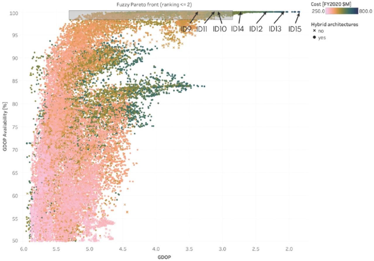
Solutions in the fuzzy Pareto front (Pareto ranking ≤ 3) shown in three-objective space (color-coded by space segment cost) with a GDOP availability metric greater than 50%. Marker shape indicates whether the architecture is hybrid (circle) or pure Walker (cross). The shaded rectangular area, shown in detail in Figure 7, contains all constellations with at most 27 satellites and producing a GDOP availability > 98%. Highlighted architectures are those in Table 3 with more than 27 satellites.
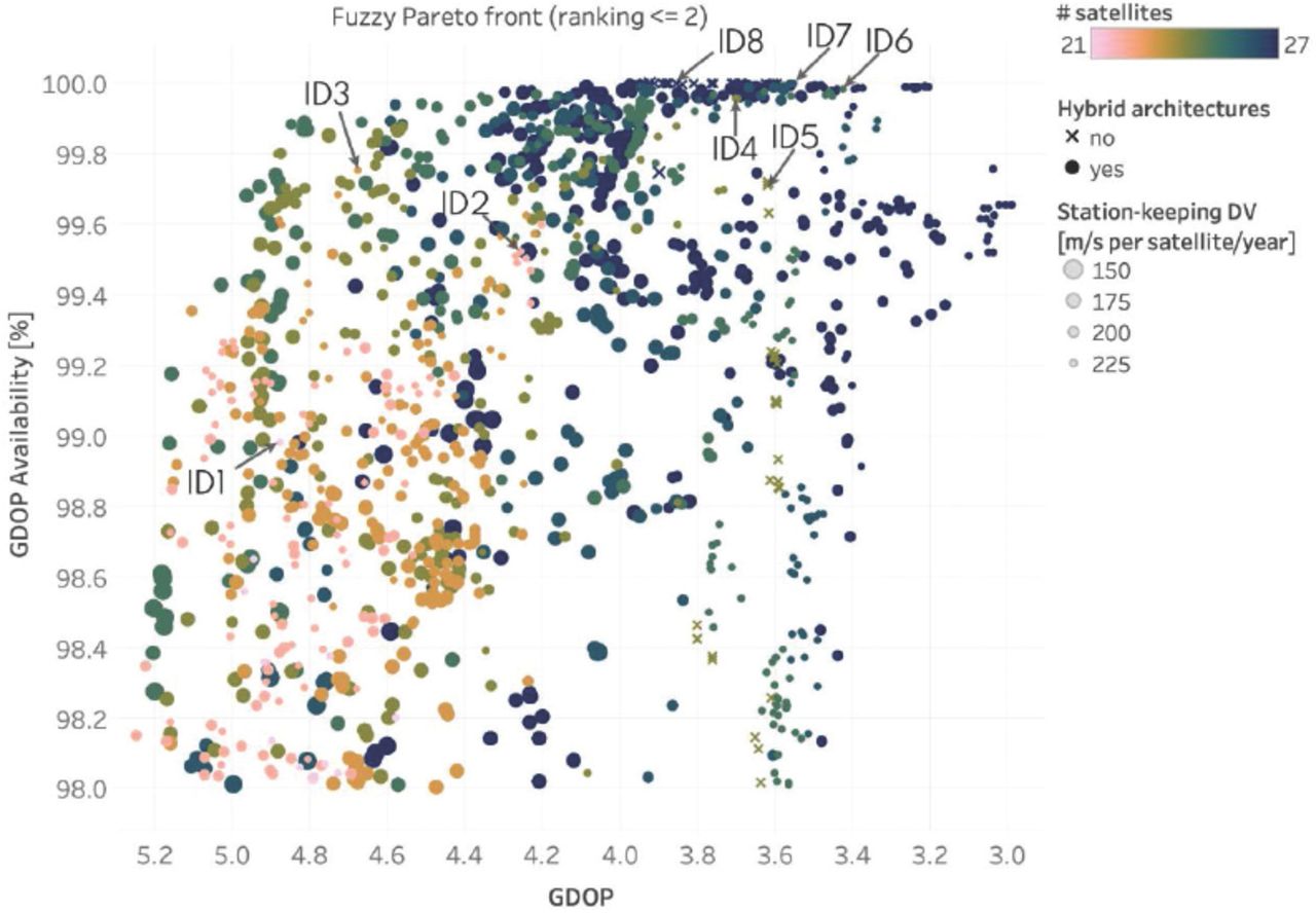
Solutions in the fuzzy Pareto front (ranking ≤ 3) with a GDOP availability greater than 98%, station-keeping ΔV < 250 m/s/sat/year, and a total constellation size of less than or equal to 27 satellites; the marker color corresponds to the total number of satellites while the marker type indicates whether the architecture is hybrid (circle) or pure Walker (cross). The marker size is proportional to station-keeping ΔV. Highlighted architectures are those in Table 3 with up to 27 satellites.
Figure 7 shows the fuzzy Pareto front architectures with ranking less or equal than three (a solution with rank I is dominated by i-1 other solutions) that produce a GDOP availability greater than 98% and station-keeping ΔV less than or equal to 250 m/s per satellite/year. The marker size is inversely proportional to the required station-keeping ΔV (grouped in bins with a resolution of 25 m/s). The marker color differentiates the total number of satellites, and the marker type is used to distinguish between hybrid (circle) and pure Walker (cross) constellations.
From Figure 7, it is apparent that most architectures in this region are hybrid and that, as expected, there is a trade-off between the number of satellites (and thus space segment cost) and GDOP performance, with best-performing solutions on the top-right corner requiring the highest number of satellites. The best GDOP performing solution (GDOP = 1.85 and GDOP availability = 100%) and one of the most expensive is a hybrid constellation with a total of 40 satellites (Arch ID 15).
Additionally, more ΔV-efficient designs are located predominantly on the left side (larger GDOP), which indicates a trade-off between ΔV-efficiency and GDOP performance. In particular, satellites in retrograde near-equatorial (orbit inclination ~178 deg) orbit are the most ΔV-efficient. Thus, hybrid designs with a few satellites in these orbits (and the remainder in polar orbit) tend to be more ΔV-efficient but exhibit worse GDOP than polar Walker designs for the same constellation size.
Pure Walker constellations shown with a cross mark are among the best solutions. The architectures highlighted with a green cross are composed of 24 satellites and constitute a reasonable compromise between constellation size (cost) and performance—although this judgment depends on the decision-maker’s willingness to pay for additional performance. Also shown are architectures with 27 satellites (blue cross), which are sufficient to achieve close to 100% GDOP availability. A common feature that emerges among the pure Walker constellations depicted in this plot is that they contain three orbital planes—eight satellites per plane (green); nine satellites per plane (blue). This feature is captured in one of the rules identified in the rule mining section.
Table 3 presents fuzzy (ranking 3) Pareto-front architectures that achieve GDOP availability 98% and a station-keeping ΔV ≤ 250 m/s per satellite/year. For reference, Architecture ID 14 is the best GDOP performing the 30-satellite Walker constellation and Architecture ID 15 is the best GDOP performing architecture overall—both of these reference designs produce a station-keeping ΔV > 250 m/s per satellite/year. Since many architectures satisfy the requirements stated above (as seen in Figure 7), Table 3 presents the solutions with best GDOP performance for different total number of satellites.
Architectures 1–13 are examples of architectures in the fuzzy Pareto front (ranking ≤ 3) that achieve GDOP availability ≥ 98% and a station-keeping ΔV ≤ 250m/s per satellite/year. For reference, Arch. ID 14 is the 30-satellite architecture with best GDOP performance. Arch. 15 is the architecture with best GDOP performance overall.
Figure 8 shows a visualization of the satellite constellation of Architecture ID 5 with 24 satellites in near-circular polar orbit and distributed among three orbital planes—a common characteristic among optimal designs.
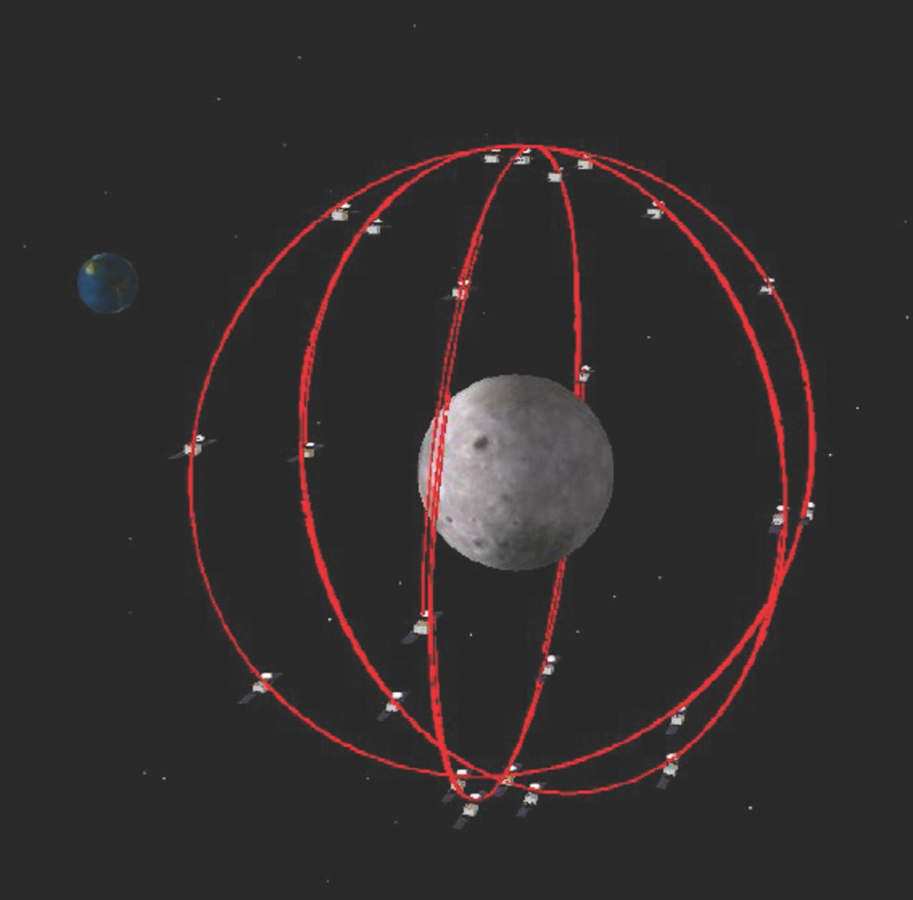
Visualization of Arch ID 5 satellite constellation (GMAT)
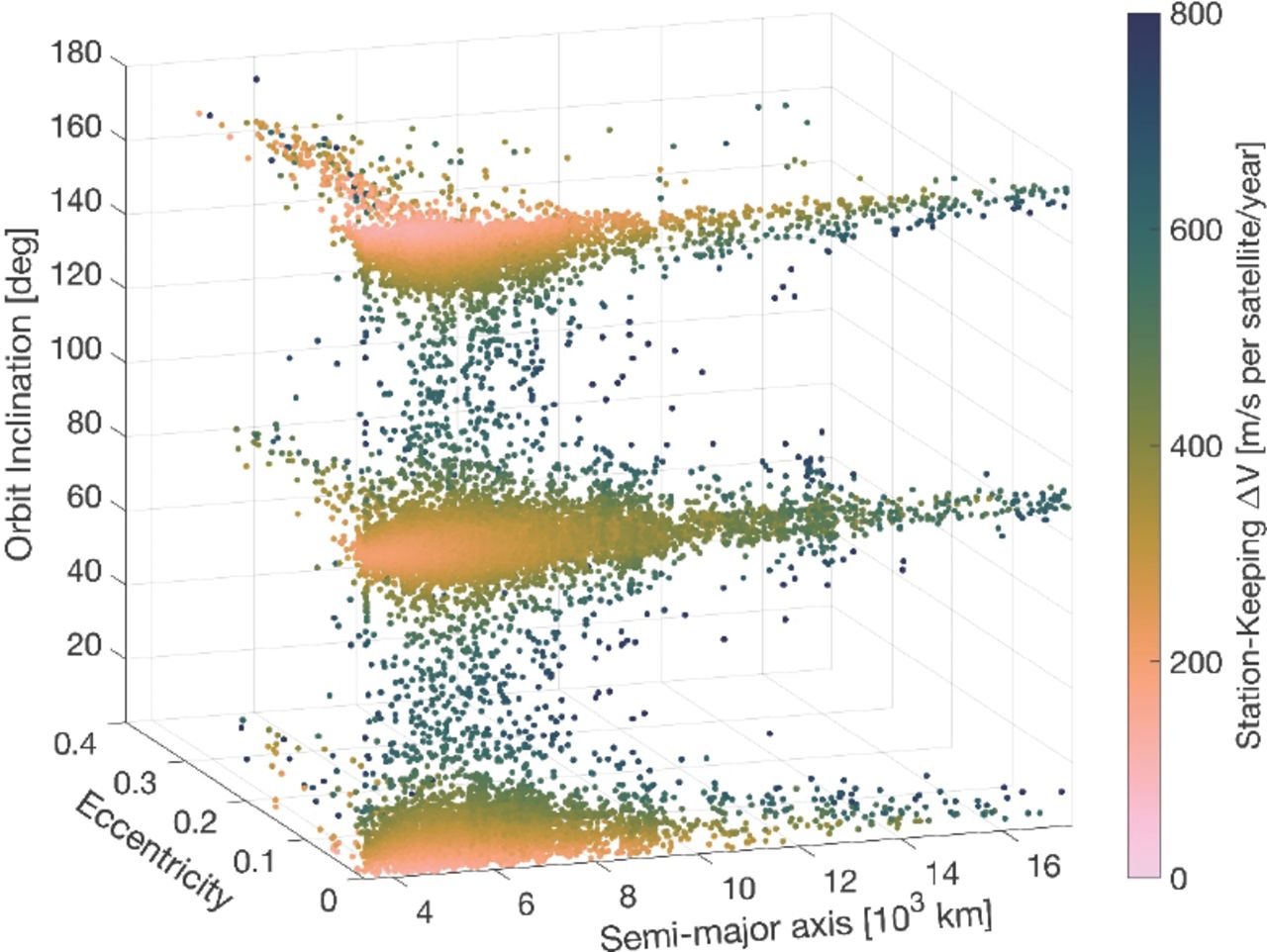
The visualization of orbital design parameters for pure Walker constellation solutions (~40,000) in design space, as shown in Figure 9, provides additional insights—hybrid solutions are excluded from the plot because different constellations in the architecture have different orbital parameters, so it is impossible to assign a single set of orbital parameters to the architecture.

Pure Walker solutions in design subspace (color-coded by station-keeping ΔV). Every dot represents a distinct architecture.
First, the algorithm converges to solutions with very small (median = 4.6 × 10⁻³) orbit eccentricity—20% of solutions have ECC < 0.01 in the first 100 function evaluations; 62% in the first 600 evaluations—which means that the optimal orbits tend to be nearly circular. Second, near-circular orbits at polar (i ≈ 90°) and equatorial (i ≈ 0°, 180°) regions are characterized by low values of station-keeping ΔV (< 300 m/s per satellite/year), especially when the semi-major axis is below 10,000 km. These observations help interpret the results and characteristics of optimal Pareto-front architectures in Table 3.
The right ascension of the ascending node (RAAN) plays a non-negligible role in the overall station-keeping ΔV budget as seen in Figure 10. For example, for Architecture ID 5, the ΔV component attributed to Δvhpole (from Equation [2]) that is used in RAAN corrections can vary from an annual 122 m/s at 90 degrees to just 10 m/s at 210 degrees RAAN. Thus, constellations with multiple orbital planes (and thus different RAANs) likely have satellites with different ΔV requirements, depending on their particular spatial orientation.

Variation of station-keeping ΔV versus orbit inclination and RAAN for a design with SMA = 5,730 km, ecc. = 5.7e-3, and AOP = 90 deg (as in Arch ID 5 in Table 3).
As mentioned in the previous section, all GDOP calculations were done for a one-year simulation period due to computational reasons, since the total number of function evaluations was very high (250,000). Figure 11 presents a map of the 98th percentile of GDOP for a few selected designs over a period of five years—and six months for comparison.

The GDOP (98th percentile) plot over the lunar surface obtained for a period of six months (240 samples) and five years (2,400 samples) for Architecture IDs 4, 5, 8, 11, and 14. Similarities between the six-month and five-year plots are an indication of effective station-keeping maneuvers.
The GDOP performance is similar in six-month and five-year periods, which means that the station-keeping maneuver sequence is able to maintain satellite geometry over a long period of time. In particular, we looked at Architecture IDs 4 and 5 (Table 3), which had the same overall number of satellites (i.e., 24 satellites), but were hybrid and pure Walker constellations, respectively.
Additionally, we looked at Architecture ID 8 (best 27-satellite Walker), Architecture ID 11 (best 30-satellite hybrid), and Architecture ID 14 (best 30-satellite Walker) to determine the impact on GDOP performance of additional satellites. The six-month plot is generated with 240 samples per grid point obtained with the LHS method, while the five-year plot contains 2,400 samples per grid point. Natural neighbor interpolation (without extrapolation) of the scattered data is used to plot the GDOP values over a plate carrée projection of the lunar surface.
The GDOP plots in Figure 11 also reveal how GDOP performance varies as a function of latitude. For example, it shows that designs containing polar orbits with at least 24 satellites tend to have great performance (GDOP ≈ 3.0) at the poles and mid-latitude regions, but exhibit poorer performance at the equator. However, hybrid designs (mixes of equatorial and polar orbits) with a limited number of satellites in polar orbit can exhibit poorer performance at the poles (e.g., Architecture ID 4’s performance over five years).
The plots in Figure 11 fail to capture the highly dynamic nature of GDOP evolution over time, which is better appreciated in video format. To quantify long-term performance more accurately, the maximum GDOP outage (GDOP > 6.0) duration is computed with a five-minute time step over one sidereal lunar month after propagating the orbit for five years.
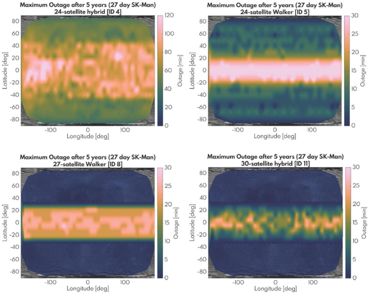
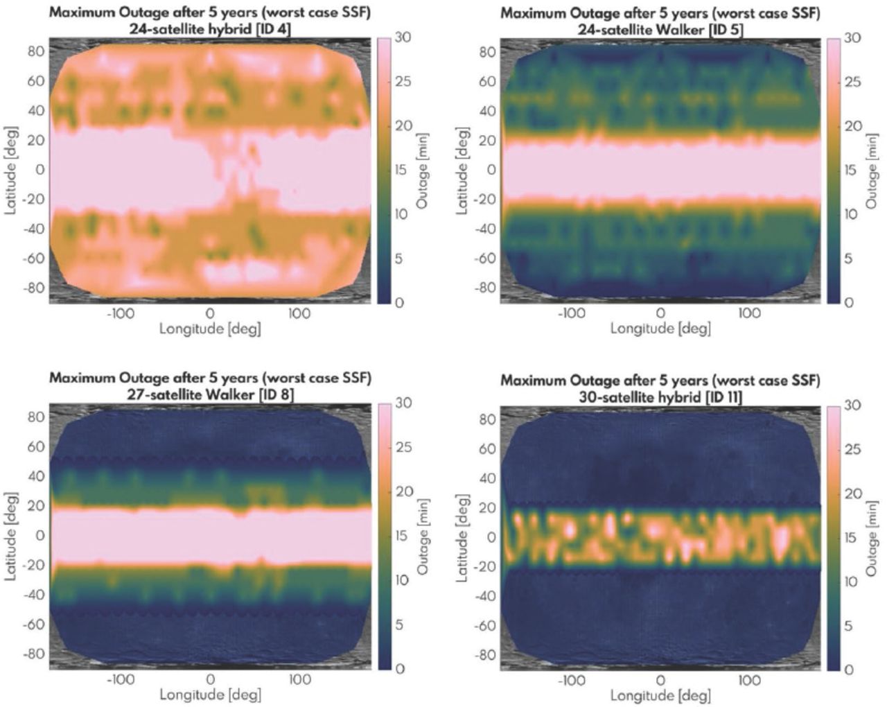
The maximum GDOP outages experienced on the lunar surface for Architecture IDs 4, 5, and 8 are shown in Figure 12. The designs with 30 satellites (Architecture IDs 11 and 14) experienced no outage over the simulation period and are therefore not shown in Figure 12.
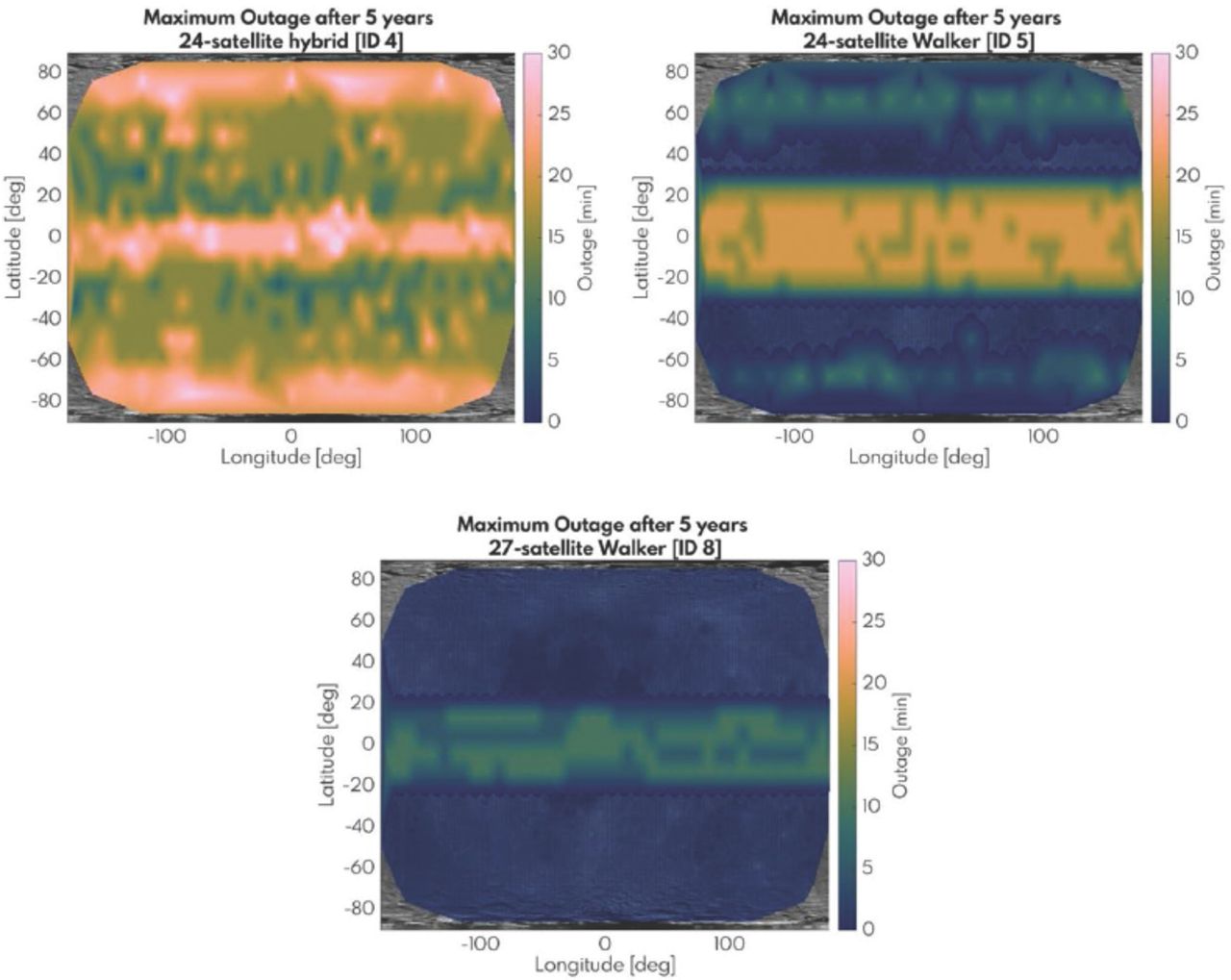
Maximum GDOP outage (GDOP > 6.0) plot over the lunar surface obtained over a one-month period after propagating orbits for five years for Architecture IDs 4, 5, and 8
Based on the results presented in Figures 11–12 and Table 3, hybrid constellations (e.g., Architecture IDs 4 and 11) have proven to be more efficient in terms of overall station-keeping ΔV—these efficiency gains can be attributed to satellites in equatorial orbits—but do not offer benefits in terms of overall GDOP performance when compared to pure Walker constellations (Architecture IDs 5 and 14). A 24-satellite Walker constellation (Architecture ID 5) exhibits worse GDOP performance at the equatorial regions with maximum outages of 20 minutes, while the hybrid design (Architecture ID 4) has poorer performance at the poles with maximum outages of 35 minutes.
The impact of worst-case single-satellite failure objectives can be used to compare the robustness of the candidate constellation IDs 4, 5, 8, 11, and 14. When comparing Figure 13 with Figure 12, it is clear that the equatorial regions are the most impacted by satellite failure. Architecture ID 14 is an interesting 30-satellite Walker design since it produces no GDOP outage.

Maximum GDOP outage (GDOP > 6.0) plot over the lunar surface obtained over a one-month period after propagating orbits for five years and considering the worst-case single satellite failure
Finally, as an example, Table 4 shows two 27-satellite Walker constellations that exhibit the best robustness to single-satellite failure objective values. These are architectures at lower inclinations—58 degrees (Architecture ID 16), which is typical of Earth GNSS constellations—or polar constellations at much higher altitude (e.g., Architecture ID 17) when compared to the best overall Walker constellation (Architecture ID 8). In the case of satellite failure, the impact on GDOP would be negligible for Architecture IDs 16 and 17. On the other hand, both of these designs required a roughly twofold increase in station-keeping ΔV.
Example of robust architectures to single-satellite failure
An incoming navigation signal in the Earth-Moon direction was used in the GDOP computation to simulate an Earth GNSS signal. The impact can be assessed by comparing Figure 11 and Figure 14 for Architecture ID 8. The largest improvement (decrease) in GDOP is seen in the regions where the signal was most geometrically diverse in relation to the available lunar GNSS signals. These regions are located at the equator at 0 degrees longitude—signal at zenith—and near the lunar surface periphery, as seen from Earth (low elevation signals).
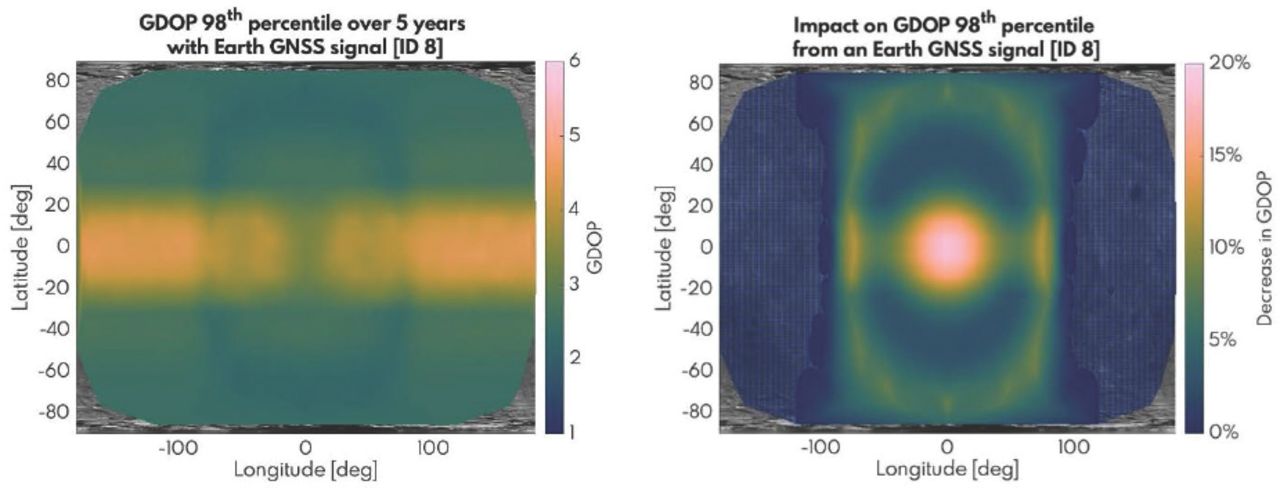
Left: GDOP (98th percentile) plot over the lunar surface obtained for a period of five years (2,400 samples) for Architecture ID 8 with an additional Earth GNSS signal; right: Percentage decrease in GDOP (98th percentile)
3.2 Scenario II – No Station-Keeping Maneuvers
Without station-keeping maneuvers, satellites are subject to periodic changes in eccentricity that result in large variations in orbit altitude, as seen in Figure 15.

Magnitude of the position vector (left), orbit eccentricity (center), and orbit inclination (right) evolution over five years for Architecture ID 20
Out of 35,000 architectures, the best GDOP-performing architectures (GDOP degradation < 1%, GDOP availability > 98%) with the lowest number of satellites are characterized by higher design SMA values when compared to the optimal designs identified in the previous scenario (see Table 5).
Example of Pareto-front architectures
GMAT simulation results show that satellites in an initial circular orbit at an SMA lower than ~9,000 km eventually crash into the lunar surface within five years. Consequently, the payload power necessary to achieve a received signal power level of at least −150 dB anywhere on the lunar surface—computed at the maximum orbit altitude observed in a five-year period—is estimated to be 557 W per satellite on average for Architecture ID 20 and 421 W for Architecture ID 21. These values are significantly higher than the required payload power for satellites in Architecture IDs 1–15, which are in the range 316–344 W.
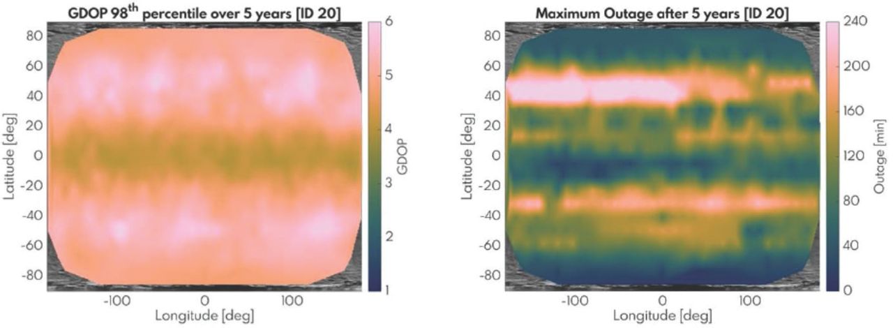
This increase in power requirement drives up satellite mass/size and space segment costs. Therefore, savings in fuel mass are offset by payload mass in the no-maneuver optimal designs and the resulting space segment costs are equivalent (to within 2–3%) to those obtained in optimal designs in the station-keeping maneuver scenario. The GDOP performance of Architecture ID 20 is considerably worse than Architecture ID 7 containing the same number of satellites, and the GDOP outage can amount to four hours in some locations as seen in Figure 16. These findings highlight the important role of station-keeping maneuvers in long-term GDOP performance.

Left: GDOP (98th percentile) plot over the lunar surface obtained for a period of five years; right: Maximum GDOP outage (GDOP > 6.0) time plot over the lunar surface obtained over a one-month period after propagating orbits for five years for Architecture ID 20
Figure 17 shows the improvement in GDOP obtained by including Earth GNSS signals, in the context of Architecture ID 20. Similarly to the results in Scenario I, users in equatorial (+/− 20 degrees longitude) and near-polar regions with an unobstructed view of the Earth can greatly benefit from such signals, provided that they can overcome the problems associated with near-far effects.

Left: GDOP (98th percentile) plot over the lunar surface obtained for a period of 5 years (2,400 samples) for architectures ID 20 with an additional Earth GNSS signal. Right: Percentage decrease in GDOP (98th percentile)
4 SENSITIVITY ANALYSIS
This section presents results from sensitivity analysis to both model parameters and design decisions that provide a deeper insight into the model. Rule mining results showing support for data patterns identified previously in optimal architectures are also presented.
4.1 Sensitivity to Model Parameters
Results from a sensitivity analysis for two important model parameters are shown below. First, sensitivity to the approximate maneuver period is assessed. To be precise, we introduced variation in the time interval (days) used to compute the average of the accumulated daily orbit errors. Since the maneuvers were not instantaneous and occurred only at specific orbital locations, the maneuver period includes the orbit propagation time to these locations. Second, the impact of increasing the degree of the lunar gravity model is assessed.
4.1.1 Sensitivity to the Satellite Maneuver Period
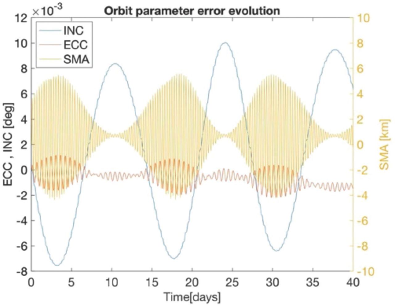
The performance of the station-keeping maneuver sequence depends on the magnitude of orbit parameter errors. The time evolution of these errors can be seen in Figure 18 for Architecture ID 14.

Time evolution of orbit parameter errors for Architecture ID 14 without station-keeping maneuvers
As discussed previously, the mean orbit error values are used directly in the computation of ΔV magnitudes and, therefore, the time period (number of days) chosen to collect the error measurements and compute the mean is an important operational parameter. Table 6 shows how the performance is affected by this parameter and its implications in terms of propellant mass, space segment cost, and design lifetime.
Effect of station-keeping maneuver frequency on station-keeping ΔV, max outage time, satellite mass, and cost for Architecture IDs 4, 5, 8, 11, and 14
A station-keeping maneuver period increase from seven to 27 days resulted in a significant reduction in the required ΔV. If we assume a fuel mass of at most 45% of the satellite wet mass (range of validity for the satellite wet mass model presented above), the maximum satellite operational lifetime—when the satellite runs out of fuel—would be limited to six years in the seven-day period and 17 years in the 27-day period case (average values for Architecture IDs 4, 5, 8, 11, and 14). Table 6 presents satellite mass and cost figures associated with a 15-year design lifetime that are feasible under the 27-day period case.
There is, therefore, an interesting trade-off between GDOP performance (seen when comparing Figures 12 and 19) and satellite mass, cost, and design lifetime. A weekly maneuver frequency is able to better maintain the satellite geometry in the long-term and thus produce better GDOP performance compared to a monthly scheme. On the other hand, this strategy resulted in a significant increase in satellite mass and reduction of design lifetime. This is assuming the absence of in-orbit refueling missions that could potentially extend the operational satellite lifetime. The results in Table 6 also show that for Architecture ID 14, despite the GDOP degradation experienced in the 27-day maneuver scheme, the GDOP outages (GDOP > 6.0) remain negligible. This is a consequence of the large number of satellites (30) in this design.
Maximum GDOP outage (GDOP > 6.0) plot for Architecture IDs 4, 5, 8, and 11, with station-keeping maneuvers every 27 days
Finally, while the strategy used in this study is able to maintain the satellite geometry over a long period of time, it is certainly possible to optimize the maneuver scheme to better exploit the periodicity of the dynamic environment for a specific constellation design.
4.1.2 Sensitivity to the Degree/Order of the Lunar Gravity Model
The sensitivity to the degree of the lunar gravity model was analyzed for Architecture ID 4—in this solution, the satellites orbited the Moon at an altitude of 3,776 km, which is representative of optimal designs. The initial settings in the LP165P gravity model were degree/order 10 of the underlying spherical harmonic expansion. Compared to the maximum degree/order (i.e., 165), we found that the maximum difference obtained in the magnitude of the satellite position vector over a period of five years was 6.3 meters. Thus, the differences in GDOP were, again, negligible.
4.2 Sensitivity to Design Decisions
The Sobol indices were computed based on 45,000 model evaluations. Figure 20 shows the first-order index and the effect of interactions (among design decisions) with the associated 95% bootstrap confidence intervals.
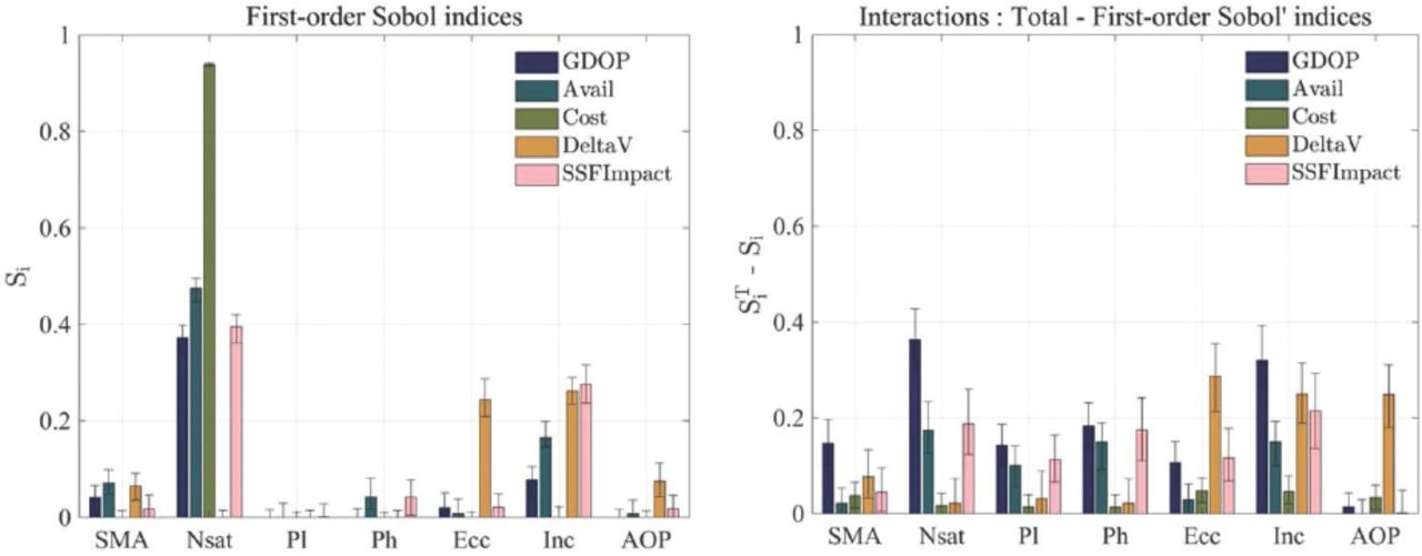
First-order Sobol index (left) and effect of interactions (right) shown for every design variable and objective metric with 95% confidence interval
The first order Sobol index plot shows that space segment cost is well-approximated by a linear function of the number of satellites, which is expected given Equation (7). Additionally, approximately 40% of the variance of GDOP performance objectives (GDOP, GDOP availability, and impact to SSF) can be attributed to variations in the number of satellites, alone. However, there are significant interactions between decision variables, which is to be expected given the complexity of the dynamic environment—this also highlights the significance of high-fidelity simulations. Finally, Figure 20 shows the relative importance of orbit eccentricity and inclination in determining station-keeping ΔV, which is consistent with the observations made previously in relation to Figure 9.
4.3 Rule Mining
This subsection presents a set of rules derived from the data set that characterizes architectures in a desired region of objective space. This region of interest is specified in terms of GDOP availability larger than 98%, station-keeping ΔV less or equal than 250 m/s per satellite/year, and a constellation size of at most 30 satellites. Furthermore, rules mined without subjective preference (involving data quartiles) are also presented.
To improve the interpretability of the rule mining results, the analysis focuses on pure Walker architectures only (design variables 1–7, as shown in Table 1). This is because aggregated objective metrics are produced in hybrid designs and the mapping between decision variables and objectives is less clear. Table 7 shows mined rules that involve antecedent design variables and consequent objective metrics with high confidence (max(conf (C → A), conf (A → C)) > 0.8).
Association rule mining results obtained for pure Walker architectures—SMA is reported in km, inclination in deg, station-keeping (SK) ΔV in m/s/sat/year, and cost in $M FY20.
As expected, more specific rules (with a higher number of conditions in the antecedent) such as Rules 1 and 2 tend to achieve higher conf(C→A) but lower conf(A→C), whereas the opposite is true for more general rules such as Rules 4 and 5. Rules 1 and 2 are the most general rules that fully explain the region of interest (which includes the fuzzy Pareto front in Rule 2) with conf(C → A) = 1. In other words, the range of values shown for the decision variables are the largest (least constraining) that still contain all solutions in the region of interest.
The high lift values for Rules 1 and 2 indicate that there is high degree of statistical dependency between A and the region of interest. The small confidence of rule (A → C) can be interpreted as A being a necessary but not sufficient condition for a solution to be in the region of interest. These results are consistent with the previous GDOP analysis and indicate that constellations with at least 24 satellites in near circular polar orbit at ~2 lunar radii are good solutions.
Rules 3–7 were chosen based on their high conf(C→A) values. Some of the rules are expected (e.g., 3, 5, and 6) but others provide additional insights. Rule 4 shows that the most SK-ΔV efficient designs are those containing satellites in a retrograde near equatorial orbit with inclination between 170 and 180 degrees. This explains the lower SK-ΔV budget of hybrid designs with satellites in these orbits when compared to same size Walker constellations (e.g., Architecture ID 4 vs Architecture ID 5). Interestingly, Rule 7 shows that a sparser constellation with 14 to 17 satellites in a near-circular near-equatorial orbit provides a relatively inexpensive and SK-ΔV efficient solution if GDOP availability is not required globally (GDOP performance at the poles would likely be very poor in this design).
5 CONCLUSION
The design space of lunar orbiting GNSS constellations has been thoroughly explored in this paper. The Borg MOEA framework was used to explore ~250,000 architectures and identify optimal designs that minimized GDOP, maximized GDOP availability, as well as minimized space segment cost, station-keeping ΔV, and impact from worst-case single-satellite failure. Results showed that a satellite constellation with at least 24 satellites distributed among three planes in a near-circular polar orbit at an altitude of ~2 lunar radii could achieve a global GDOP of six or less 98% of the time. The impact of single-satellite failure on GDOP was lower both for constellations at higher altitudes and with orbit inclinations typical of Earth GNSS (i≅58 deg), however these designs were penalized with a twofold increase in station-keeping ΔV when compared with the multi-objective optimal solutions.
Trade-offs are evident between overall GDOP performance and space segment cost/station-keeping ΔV. Also, it is shown that a 24-satellite Walker constellation (Architecture ID 5) could produce great GDOP performance (GDOP < 3) at the poles—where scientifically important sites, such as the South Pole Atkins Basin, are located—with minimal outages even in case of SSF. However, for this constellation, users at equatorial regions would see GDOP outages (GDOP > 6.0) of up to 20 minutes (40 minutes in case of SSF). A sensitivity analysis showed that the main factor in GDOP performance (including availability and robustness) was the number of satellites. Architectures with 30 satellites (e.g., Architecture ID 14) could effectively eliminate GDOP outages globally.
The optimal hybrid constellations consisted of a mix of equatorial and polar orbits; however, no significant advantages were observed compared to pure Walker constellations with the same number of satellites—in part due to the worsening performance at polar regions.
The importance of the station-keeping maneuver strategy in long-term performance is highlighted. In particular, trade-offs between station-keeping maneuver periods of one week and 27 days (approximately one sidereal lunar month) were presented for several alternative architectures. In the seven-day case, the best designs required a ΔV of ~250 m/s per satellite/year. On the other hand, the 27-day case resulted in a degradation of GDOP (especially for constellations with less than 30 satellites) but allowed for a threefold decrease in fuel mass and threefold increase in design lifetime—under the assumptions that fuel mass does not exceed 45% of satellite wet mass and that the satellite may not be re-fueled in orbit.
Under a no-station-keeping maneuver scenario, optimal solutions showed a ~25% degradation in overall GDOP performance (with GDOP outages up to four hours) and did not result in significant mass or cost savings compared to the case with station-keeping maneuvers. These solutions undergo large periodic variations in eccentricity over a five-year period and, therefore, require more radiative power at apoapsis to guarantee the same signal power level on the lunar surface. The mass gains due to fuel savings are thus offset by mass penalties caused by the additional payload mass (assuming payload power generation drives payload mass estimates).
The final positioning accuracy achieved with the proposed lunar GNSS depends on the signal-in-space range error (SISRE), instantaneous GDOP at the user location, and quality of the signal processing techniques. Yet, based on recent results (Hauschild & Montenbruck, 2021), we believe that to achieve the target position accuracy (< 0.4 m), a SISRE of 0.5 m (RMS) is an appropriate goal for lunar GNSS ground segment design.
5.1 Limitations
There are several limitations in this article. First, the ΔV computation neglects satellite orbit insertion and ADCS maneuvers (e.g., antenna pointing, reaction wheel off-loading). Second, parametric models for mass and cost were based on historical data from communication and navigation satellites in Earth orbit. The cost model ignored sources of cost such as control segment and operational costs.
Third, satellite phasing and constellation symmetry were constrained to a Walker delta pattern, which despite its widespread use in Earth orbiting constellation design, effectively excludes other potential interesting designs. It may be valuable to consider using RAAN as a design variable given the observed variations in station-keeping ΔV as a function of this orbit parameter orientation. Fourth, a spherical satellite body was assumed for determining the effects of solar radiation pressure, which is only valid as a first approximation. Finally, we do not consider more than two constellations in hybrid designs.
5.2 Future Work
It would be interesting to complement the findings in this work with control segment design and analyze the trade-offs between signal-in-space error (orbit and clock synchronization errors) and overall system cost. Important considerations exist regarding the implementation of system time and how to best synchronize the master clock with other time references on Earth. This work could be used toward the definition of a lunar GNSS service over a period of time (e.g., 30 years) to effectively extend the GNSS space service volume to the Moon’s vicinity.
Thus, the proposed constellations would constitute the target configurations at full operation capability. The optimization of service quality over time could be achieved by analyzing trade-offs in the gradual deployment of space and control segment elements. In this context, it would make sense to conduct an epoch-era analysis (Ross & Rhodes, 2008) including strategies for orbit determination, Earth-lunar GNSS time transfer, satellite launch timeline, orbit evolution policies, and the integration of new technology.
HOW TO CITE THIS ARTICLE
Pereira, F., Reed, P. M., & Selva, D. (2022) Multi-objective design of a lunar GNSS. NAVIGATION, 69(1). https://doi.org/10.33012/navi.504
ACKNOWLEDGMENTS
The authors would like to thank Jean-Luc Issler for useful comments regarding ITU regulations as well as the ITU and SFCG recommendations in the shielded zone of the Moon.
- Received February 26, 2021.
- Revision received October 8, 2021.
- Accepted November 13, 2021.
- © 2022 Institute of Navigation
This is an open access article under the terms of the Creative Commons Attribution License, which permits use, distribution and reproduction in any medium, provided the original work is properly cited.


Jump to section
Related Articles
Cited By...
- No citing articles found.