

Abstract
Applications of precise point positioning (PPP) are limited by PPP’s long convergence time. One effective way to shorten the convergence time is to apply ionospheric constraints because of the external ionospheric information. The conventional way to do this is to apply high precision but biased ionospheric corrections. The limitations of the method are that all ionospheric constraints must be derived from the same set of reference stations to have the same data. An approach based on single differences between satellite ionospheric constraints (SDBS-IONO) is developed to address the data issue due to having no common satellite visibility. The proposed method is more flexible and scalable in terms of adding ionospheric constraints. Based on a network of about 130 stations, we validated the proposed SDBS-ION method and compared it to the conventional method. Our results confirm that the ionospheric constraints enhance the PPP convergence time significantly depending on the accuracy of ionospheric constraints. Finally, we discuss crucial factors regarding how long and accurate the effectiveness of ionospheric constraints are in reducing PPP convergence time.
- between-satellite ionospheric constraints
- biased ionospheric observables
- constrained UPPP model
- precise point positioning (PPP)
- SDBS-ION
- uncombined PPP (UPPP)
1 INTRODUCTION
Based on a standalone receiver, the precise point positioning (PPP) technique has become popular due to its cost-effectiveness and operational flexibility (Héroux & Kouba, 1995; Zumberge et al., 1997). However, PPP suffers from a long convergence time, taking 15 to 60 minutes to reach centimeter-level positioning accuracy (Bisnath & Gao, 2008), which significantly limits its applications. The PPP convergence time is attributed to several factors, including pseudorange noise level, error corrections, geometry of visible satellites, receiver environment, receiver dynamic, and data quality. Correspondingly, PPP ambiguity resolution, multi-GNSS, multi-frequency, and PPP-RTK (real-time-kinematic) have been investigated to enhance PPP performance (Cai & Gao, 2013; Collins et al., 2010, 2012; Ge et al., 2008; Geng & Bock, 2013; Laurichesse et al., 2009; Leandro et al., 2011; Nie et al., 2019b; Seepersad & Bisnath, 2015; Teunissen & Khodabandeh, 2015).
Among the mentioned methods, PPP-RTK exploits the external atmosphere information from regional reference networks to shorten convergence time. Atmosphere information consists of tropospheric corrections and ionospheric corrections. The tropospheric corrections are accurate at the millimeter-to-centimeter level. For example, Shi et al. (2014) improved the positioning accuracy by delivering tropospheric corrections at an accuracy of around 1.4 cm in a one-way direction from a server to users. They achieved a positioning accuracy of 9.2 cm for the horizontal component and 10.1 cm for the vertical after 20 minutes’ convergence, in contrast to 14.7 cm and 21.5 cm without augmentation.
Unlike tropospheric corrections, ionospheric corrections are highly correlated to frequency-related hardware biases. The conventional way to obtain ionospheric corrections is to model the ionospheric vertical total electron content (VTEC) to separate hardware biases from VTEC (Li et al., 2015; Mannucci et al., 1998; Schaer et al., 1995). However, the ionosphere VTEC is influenced by modeling and mapping errors which would degrade the accuracy of ionospheric corrections. Therefore, it is challenging to acquire accurate ionospheric corrections to meet the requirements of PPP-RTK.
Several studies have explored ways to correct ionospheric errors in PPP (Hernández-Pajares et al., 2011; Liu et al., 2018; Nie et al., 2019a; Psychas & Verhagen, 2020; Sieradzki & Paziewski, 2016; Zhao et al., 2019; Zhou et al., 2020). Among ionospheric corrections, the slant total electron content (STEC) provides highly accurate ionospheric corrections. Li et al. (2011) applied the combined atmospheric corrections from a regional network into PPP, achieving instantaneous ambiguity resolution.
Zhang et al. (2011) introduced the uncombined PPP-RTK concept, taking advantage of regional reference networks. Shi et al. (2012) enhanced the performance of single-frequency PPP by modeling the ionosphere with a polynomial for each satellite. Lou et al. (2016) studied multi-GNSS PPP by extending the ionospheric modeling. Rovira-Garcia et al. (2015) achieved fast PPP by constraining the absolute slant ionospheric corrections. Psychas and Verhagen (2020) evaluated the performance of PPP-RTK at different scales of networks. Banville et al. (2014) accelerated the convergence time with global ionospheric maps (GIMs) and a 150-km network. They also pointed out the crucial issue of coping with receiver biases, but they did not expand on this in detail.
Unlike absolute troposphere corrections, the ionospheric delays are correlated with satellite and receiver differential code biases (DCBs). The biases from the external ionospheric constraints pose a challenge when adding the ionospheric constraints for reducing convergence time. A few scholars have investigated ways to handle the biases in the ionospheric constraints. Zhang et al. (2013) and Tu et al. (2013) showed that receiver DCBs have substantial effects on convergence time in the ionosphere-constrained PPP model. Xiang et al. (2020) further analyzed how receiver DCBs have the opposite effect on code and phase measurements, as well as different scale effects on different frequencies.
Psychas and Verhagen (2020) later estimated receiver DCBs with the presence of ionospheric corrections at the user end. Zhou et al. (2020) applied predicted GIMs and estimated the receiver DCBs in the uncombined PPP (UPPP) model to obtain unbiased ionospheric corrections. Therefore, it is not difficult to see that handling the receiver biases in ionospheric constraints is crucial.
However, estimating the receiver biases requires common satellite visibility from all the same reference stations. In this study, we aim to address the issue by creating single-difference between-satellite ionospheric constraints (SDBS-ION). The method is more flexible to add external ionospheric constraints when the ionospheric constraints do not have common visibility from the same set of reference stations. Positioning tests were performed to illustrate its effectiveness.
The paper is organized as follows: Section 2 illustrates adding direct but biased ionospheric constraints, and the proposed SDBS-ION method; Section 3 discusses the results of the basic and the two constrained PPP models. The proposed SDBS-ION method is also compared with the direct but biased ionospheric constraints using 130 stations. Finally, in Sections 4 and 5, key factors on ionospheric constraints are discussed, and conclusions are drawn briefly.
2 METHODOLOGY
We start the section with the uncombined PPP (UPPP) model and then explain two methods applying the ionospheric constraints to PPP. Different from the traditional PPP formulating an ionosphere-free combination, the UPPP model treats the ionospheric delays as unknown parameters (Xiang et al., 2019; Zhang et al., 2012). The advantage of the UPPP model is that the ionospheric parameters can be constrained or corrected when the external ionospheric information is available. The UPPP model can be described as:
 1
1
where Pj and Φj are code and carrier phase measurements at frequency j (j=1, 2) with a unit of meters (m); ρ is the geometry distance between receivers and satellites (m); c is the light speed; the superscript r and s refer to a receiver and satellite; dtr represents the receiver clock with the unit of seconds (s); dts represents the satellite clock (s);  and
and  are the receiver and satellite code biases for ionosphere-free combination; T represents the tropospheric delay (m);
  represents the ionospheric delay along a line of sight at the L1 frequency (m);
  represent the receiver- and satellite-related differential code biases (DCBs) (m);
  represents the float ambiguity including biases at frequency j (cycle); λj is the wavelength at frequency j (m); and εP and εΦ contain the multipath and measurement noise for code and carrier-phase measurements respectively (m). Other errors are corrected according to Petit and Luzum (2010), such as phase windup, antenna correction, Earth displacement, and relativistic effects.
The unknown parameters are estimated as follows:
 2
2
where xyz is the unknown coordinates;  contains both cdtr and
  ; T represents the vertical tropospheric delays;
  represents the slant ionospheric parameters, which consist of the satellite and receiver DCBs. This is also known as ionospheric observables, expressed as:
 3
3
2.1 Deterministic and Stochastic Models of Ionospheric Corrections
Before applying ionospheric constraints, one noteworthy consideration is how the errors of ionospheric constraints propagate from reference stations to users. Ionospheric errors are spatially related. The errors of the ionospheric constraints grow with the increase in distance between a rover station and a reference station.
The deterministic part of ionospheric constraints is interpolated from the estimated ionospheric observables based on reference stations. As satellite DCBs can be calibrated with an accuracy of 0.1 ns (i.e. 3 cm [Xiang & Gao, 2017]), the satellite DCBs can be corrected ahead using DCBs products. After correcting the satellite DCBs, the ionospheric corrections can be calculated using the inverse distance weighted method when nearby reference stations are involved.
 4
4
where i is the index of involved reference stations; xion represents the interpolated ionospheric delay at the user station; wi is the weight for each line-of-sight ionospheric observable;  represents the external ionospheric constraints from reference station(s); di is the distance between the rover and the reference stations; and
  represents the DCBs from reference station(s). As we can see from the equation, DCBs are an unseparated part of the external ionospheric constraints
  . Besides, previous studies have shown that receiver DCBs are time-variant (Zhang et al., 2019), therefore it is crucial to handle the receiver DCBs properly.
The stochastic model of ionospheric constraints consists of two parts. One part includes the formal precision depending on the measurement noise and multipath errors; the other consists of interpolated errors. We assume this uncertainty increases linearly with the distance between users and reference stations. For example, with an empirical assumption of the ionospheric errors at 0.61 mm-per-km, the standard deviation for a reference station at 100 km is 0.61 *100 mm (i.e., 0.061 m). This empirical value depends on ionospheric conditions. The variance of ionospheric constraints is calculated as follows:
 5
5
where Pion is the variance of the interpolated delays;  is the formal precision of the estimated ionospheric parameters, which is usually at centimeter-level; β is the empirical value; and el is the elevation.
2.2 Ionospheric Constrained PPP Models
We then applied the ionospheric constraints to user ends to shorten the convergence time of PPP. Two approaches to apply the ionospheric constraints as pseudo-measurements in the filter are illustrated in Figure 1. The first shows applying the direct-but-biased STEC, and the second shows the single difference of between-satellite ionospheric constraints (SDBS-ION).

Applying ionospheric constraints from the server end to a user end
First, ionospheric observables with biases from networks are applied directly. When the external ionospheric observables are applied directly to constrain the  in the user end, the receiver DCBs in ionospheric constraints become crucial, as shown in Equation (4). The reason is that the receiver DCB has a different effect on the code and phase measurements and different frequencies. This demonstrates that the receiver DCBs cannot be absorbed fully by any other parameters. An extra parameter for the receiver DCBs is needed. The unknown parameters with additional receiver DCBs when applying direct ionospheric constraints are as follows:
 6
6
where  is the estimated ionospheric parameters under constraints and
  is the additional parameter to absorb receiver-related biases. Here ex is used to distinguish this equation from Equation (2).
A disadvantage to this estimation method is that all ionospheric constraints must be derived from the same set of reference stations so the receiver bias can be absorbed into an additional parameter. Otherwise, the averaged biases could not be absorbed into an additional receiver DCB parameter. It is a strict criterion to have ionospheric observables from all reference stations to create the same benchmark. If an ionospheric constraint is not from the same set of reference stations, a trade-off between selecting the common satellite visibility and abandoning the constraint has to be made.
Secondly, the SDBS-ION method was applied. The SDBS-ION method eliminates the receiver DCBs before applying the constraints so that the state vector would remain the same when using the SDBS-ION method. In contrast to the first method requiring the same benchmarks or common visibility from the same reference stations, it is more flexible to apply the SDBS-ION constraints. The constraints of SDBS-ION can be expressed as Equation (7):
 7
7
where  represents the ionospheric observables of reference satellite at epoch t and the satellite with the highest elevation is chosen as the reference;
  represents the ionospheric observables for other satellites;
  is the between-satellite ionospheric residuals; and
  represents the DCBs between the reference satellite and other satellites.
As receiver DCBs are mitigated by creating the single difference between satellites, what remain are the between-satellite ionospheric residuals and DCBs,  . By calibrating
  and assuming the ionospheric constraints are independent of each other, we further formulated the ionospheric constraints in Equation (8):
 8
8
The variance-covariance of the SDBS-ION method, PSDBS–ION is:
 9
9
Here Pion is the variance of estimated ionospheric observables from each reference station.
In summary, these two methods shall generate similar solutions if receiver DCBs are modeled as white noise. The direct-but-biased ionospheric constraints need to model one more parameter of receiver DCBs, whereas the SDBS-ION method sacrifices one constraint when forming single differences between satellites. The advantage of the SDBS-ION method is that it is more flexible when ionospheric constraints from certain reference stations are not available.
3 RESULTS AND DISCUSSION
This section presents the data collection and validates the proposed method. First, the data set and strategies of processing data are described. We then discuss the results of basic PPP and constrained PPP in terms of estimated ionospheric observables and hourly PPP position solutions. Position accuracy and convergence time are utilized to quantify performance.
3.1 Data Set and Processing Strategies
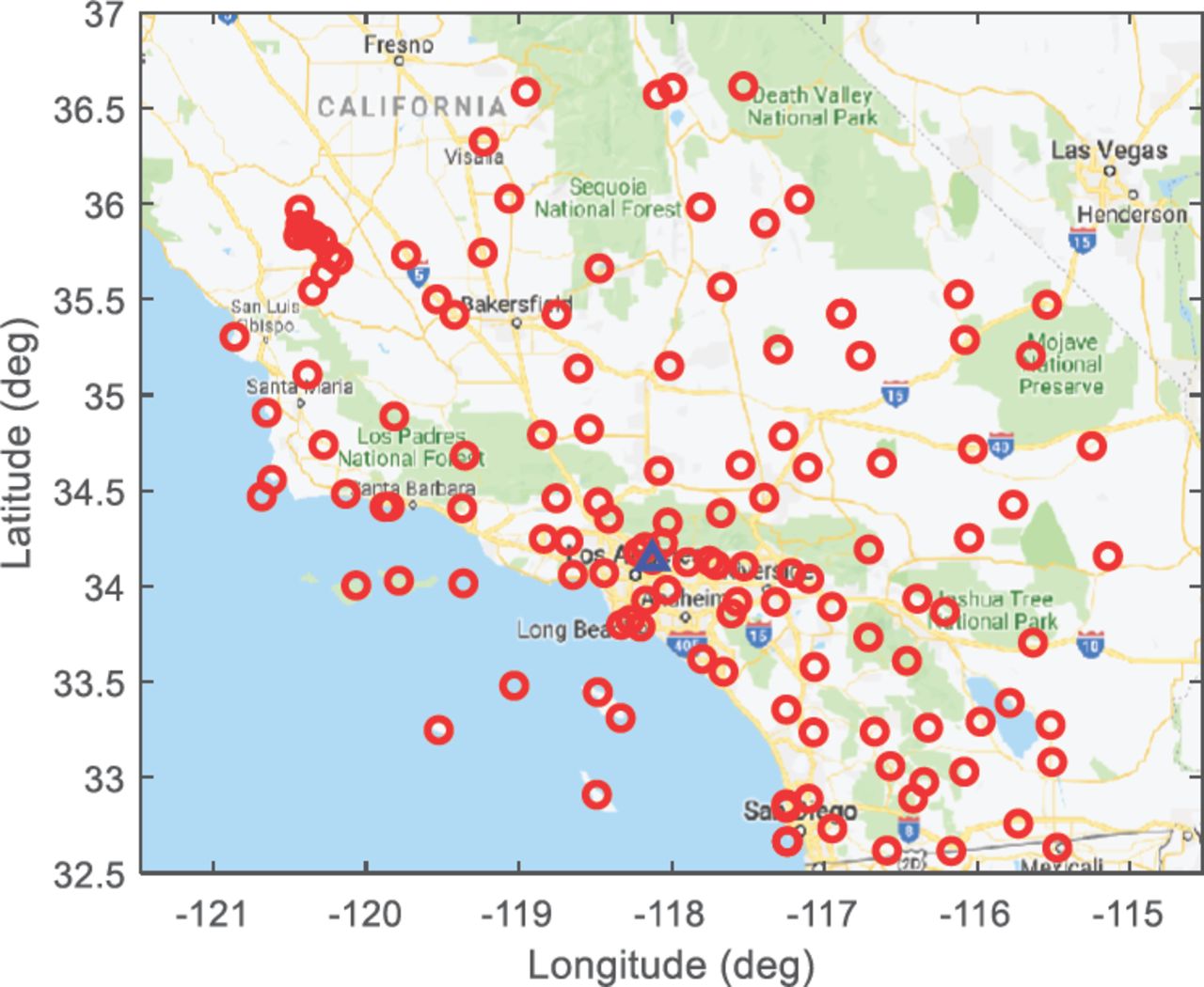
We selected about 130 stations in a year of high solar activity and a quiet day on March 16, 2015, from the U.S. continuously operating reference stations (CORS) deployed in southern California. The data are available at https://geodesy.noaa.gov/corsdata. Station CIT1 is chosen as the test (user station) to assess the biased ionospheric constraints from other stations at different distances. These stations are within a range of 300 km relative to station CIT1. The geographic distribution of all the stations is exhibited in Figure 2.

Geographic distribution of the selected 130 stations in red circles; test station CIT1 is represented using a blue triangle.
For PPP processing, the final products of both satellite orbits and clocks from the Center for Orbit Determination in Europe (CODE) are applied. The parameters and settings remain the same when comparing the constraints of direct ionospheric observables and the SDBS-ION methods. For example, the same elevation mask and the same variance threshold are required when applying ionospheric constraints. In the study, 10 degrees is chosen as the elevation mask, and the constraints are applied only when the formal precision is smaller than 0.1 m. It is worth mentioning that the DCBS are between P1 and P2. C-code measurements are aligned to P-code by correcting the corresponding bias products.
The ionospheric constraints are estimated from the UPPP for its high precision (Xiang et al., 2019). We evaluated only the data after a 4-hour convergence to make sure the ionospheric observables had effectively converged (i.e., 5:00–24:00 UTC). At the user end, CIT1 was initialized hourly. Therefore, each station had 20 sessions daily. Also, as the study focused on ionospheric effects, only the ionospheric constraints were added and no tropospheric constraints were applied. The PPP performance would be further enhanced if tropospheric constraints were applied, especially in the vertical direction (Shi et al., 2014).
3.2 Evaluation of Ionospheric Corrections
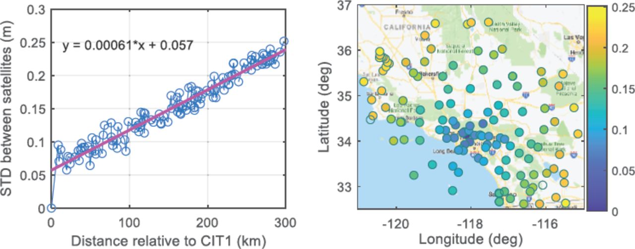
Choosing CIT1 as a user, we displayed the accuracy of the ionospheric residuals between satellites for the other 130 stations. The standard deviations (STDs) of between-satellite ionospheric residuals and their geographic distribution is shown in Figure 3. It can be seen that the STDs indicate high relevance to the distance. This means that distance is a significant factor in terms of the STEC accuracy. As shown in Figure 3, the STDs are fitted linearly as a function of distance. The incline rate is 0.61 mm-per-km. This empirical value will be applied to calculating the uncertainty of ionospheric corrections. It is worth noting that the empirical value depends on various ionospheric conditions.

STDs of the SDBS-ION method for each station against the distance to station CIT1 and the geographic distribution of the STDs for single differences between satellites
3.3 Results on the Basic UPPP Model
The estimated ionospheric parameters at CIT1 using the basic UPPP model without any constraints are given in Figure 4. The ionospheric observables change smoothly within a scale between two to 10 meters. On the left, the beginning of ionospheric observables is noisier, and ionospheric observables at the beginning are more obvious than a satellite appearing in the middle of re-convergence. The other panel of Figure 4 illustrates its corresponding formal precision. The formal precision reduces from a meter to centimeters. The noisier ionospheric observables at the beginning are also reflected in the larger formal precision. And the formal precision for the satellite appearing in the middle presents a smaller formal precision from 0.5 m compared with the beginning from 1.5 m, such as around UTC 12.9.
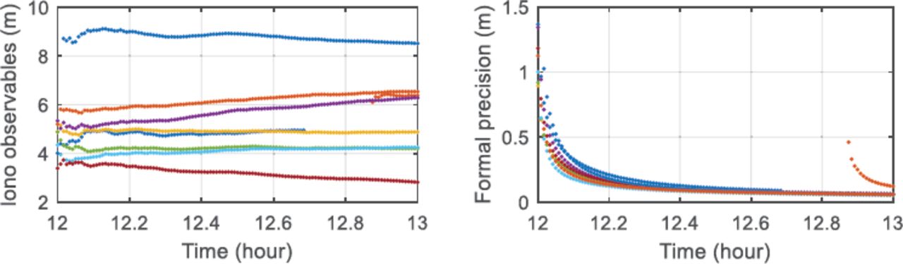
Time series of ionospheric observables and the corresponding formal precision estimated in the basic UPPP model; each color represents each satellite.
Figure 4 presents the hourly position errors of CIT1 on March 16, 2015, based on the basic UPPP model, compared to the reference coordinates based on the daily static solutions. Each hour has a new initialization because the sessions are processed every hour. Figure 5 illustrates the position accuracy in horizontal two-dimensional (2D), vertical, and three-dimensional (3D) accuracy. The convergence time to 0.1 m at the horizontal and 0.2 m at the vertical were 30.7 and 13.7 minutes, respectively. On average, the hourly position errors of the basic PPP for 2D and 3D for an hour session were 0.224 and 0.368 meters. This average of position errors and convergence time are utilized to compare with the proposed method below.

Time series of position errors at horizontal, vertical, and 3D accuracy of CIT1 on March 16, 2015, based on the basic UPPP model; sessions were processed every hour.
3.4 Results on the Constrained UPPP Model with Direct-but-Biased Ionospheric Observables
We randomly selected a station AZU1 21.3 km away to exhibit the direct ionospheric constrained UPPP model. Applying the constraints of the ionospheric observables from station AZU1, we displayed the estimated ionospheric observables at CIT1 in Figure 6. The ionospheric observables ranged from −17.5 to −15 meters, which was different from the basic UPPP model, ranging from two to 10 meters as shown in Figure 4.

Time series of ionospheric observables and the corresponding formal precision estimated in the direct-but-biased ionospheric constrained UPPP model. In the right panel, the yellow cross line on the right axis represents the corresponding elevation to the satellite in the upper blue line.
The differences were likely due to the biased ionospheric constraints from station AZU1. On the right, it is prominent that formal precision reduced faster than that from the basic UPPP model. However, one satellite in light blue was larger. We found that this satellite was not constrained. This satellite at a low elevation of around 10 degrees and the ionospheric observables from the reference station were not available. Besides, the elevation for this satellite is shown in the yellow line.
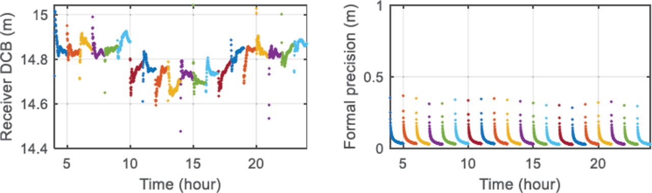
As mentioned in Section 2, receiver DCBs need to be estimated properly when applying direct-but-biased ionospheric constraints. Figure 7 displays the receiver DCBs estimated in the constrained UPPP model. The receiver DCBs are modeled as the random walk epoch by epoch. It can be noticed that the receiver DCBs diverge around 14.8 m. The right side shows the formal precision of the estimated receiver DCBs. The formal precision of receiver DCBs decreased from 0.4 m to the centimeter level.

Receiver DCBs and the corresponding formal precision estimated in the direct-but-biased ionospheric constrained UPPP model; each color represents each satellite.
The hourly position errors based on the directly constrained UPPP model compared with that of the basic UPPP model are shown in Figure 8. The blue lines refer to the direct-but-biased ionospheric constrained UPPP model and the red one is the previous basic UPPP model. It was observed that the position errors constrained using the biased ionospheric observables were much smaller than the UPPP model without any constraints. Concerning the horizontal accuracy, it is likely to reduce the initial accuracy to 0.5 meters immediately. Generally, the position errors for 2D and 3D for an hour session are 0.095 and 0.223 meters. The position errors in the east and north directions had an improvement at 62.2% and 49.4% compared to the basic UPPP model. The convergence time improved from 30.7 to 15.5 minutes horizontally (50.2% improvement), but slightly worse at the vertical in this case.
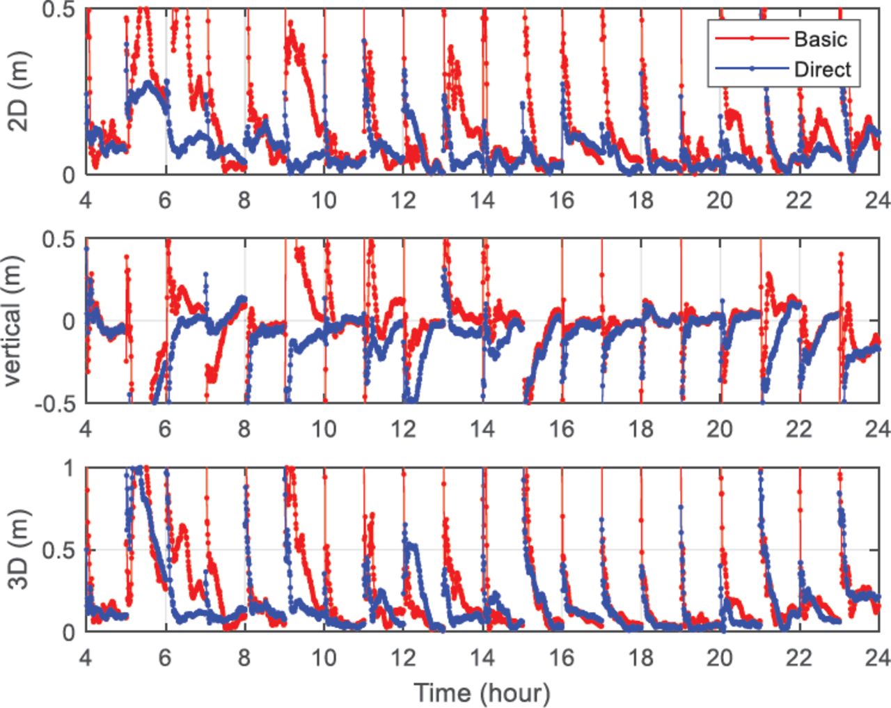
Time series of position errors at horizontal, vertical, and 3D accuracy of CIT1. The red represents the basic UPPP model. The blue is from the constrained UPPP model with the direct-but-biased ionospheric observables.
3.5 Results on the Constrained UPPP Model with the SDBS-ION Method
Comparing with the direct-but-biased ionospheric constrained UPPP model, we implemented the SDBS-ION constrained UPPP model. The estimated ionospheric observables using the proposed method are displayed in Figure 9.
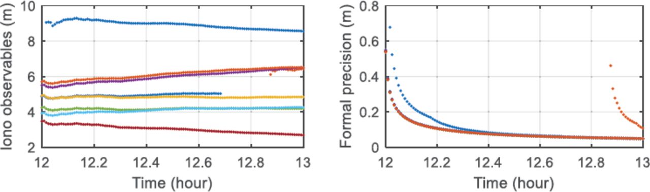
Time series of ionospheric observables and the corresponding formal precision estimated in the SDBS-ION constrained UPPP model
Compared to the ionospheric observables in Figure 4, the ionospheric observables shown here are at a similar scale, ranging from two to 10 meters. As mentioned before, this is because the SDBS-ION constraints are relative, and no more biases were introduced. The right panel of Figure 9 displays its corresponding formal precision of the ionospheric observables. It looks like only three colors are visible because the formal precisions overlapped with each other due to similar constraints. The formal precision also improved compared to the basic UPPP model, but was not as good as the direct constraints. We think the estimated receiver DCBs in the directly constrained UPPP model absorbed the uncertainty.
The position errors of the SDBS-ION constrained UPPP model with station AZU1 are displayed in Figure 10. The position performances using these two methods are similar; the average position errors for 2D and 3D for the hourly session were 0.105 and 0.236 meters, respectively. The solutions had little difference compared to the directly constrained model.
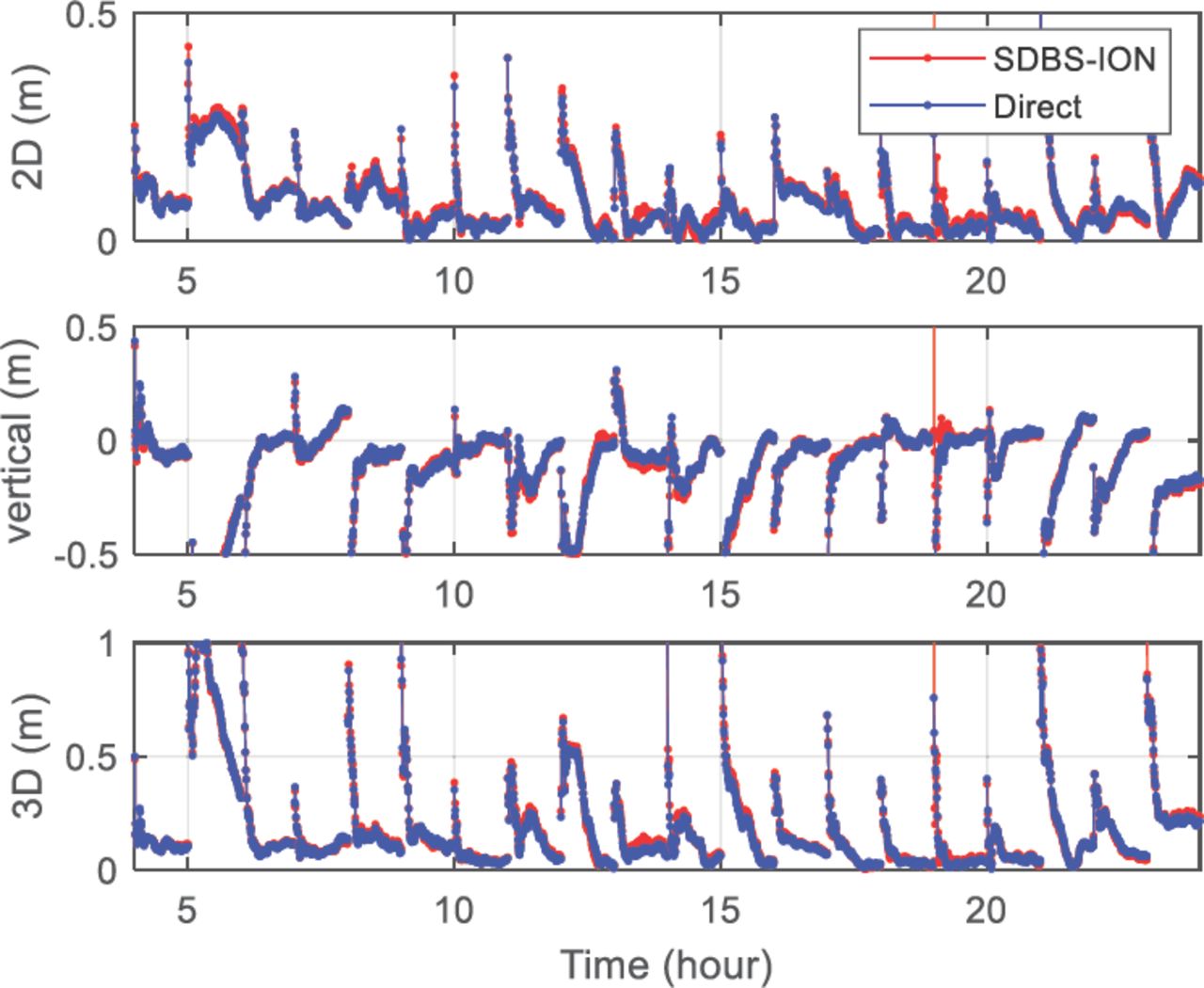
Time series of position errors at horizontal, vertical, and 3D accuracy of CIT1; the red is from the directly constrained UPPP model, and the blue is from the SDBS-ION constrained UPPP model.
3.6 Comparison of the Two Constraint Approaches
As mentioned in the data description, CIT1 was chosen as the primary test station of the 130 stations within 300 km. We utilized these 130 stations to compare the two ionospheric constrained methods and examine how effective the ionospheric constraints were at different distances.
Given the constraints of the ionosphere information from each reference station, Figure 11 shows the 2D and 3D position errors for these 130 stations using these two methods with different distances. The lower two lines with marks are the 2D position errors and the other upper two lines denote the 3D position errors. The two horizontal dashed lines are the average 2D and 3D root mean square (RMS) of the basic model. All the position errors are smaller than the basic PPP model in horizontal dashed lines. The differences between the two ionospheric constrained methods are minimal. Besides, the position errors tended to increase with the distance relative to the test station CIT1.

2D and 3D position errors for CIT1 using the direct ionospheric constraints and SDBS-ION constraints at different distances
The convergence time to 0.1 m horizontally and 0.2 m vertically using the two ionospheric constrained methods is shown in Figure 12. The two dashed red and blue horizontal lines are the convergence time of the basic UPPP model. Horizontally, the convergence time to 0.1 m using ionospheric constraints was smaller than the basic model only when the distance was less than 100 km, and the convergence time became longer afterward.
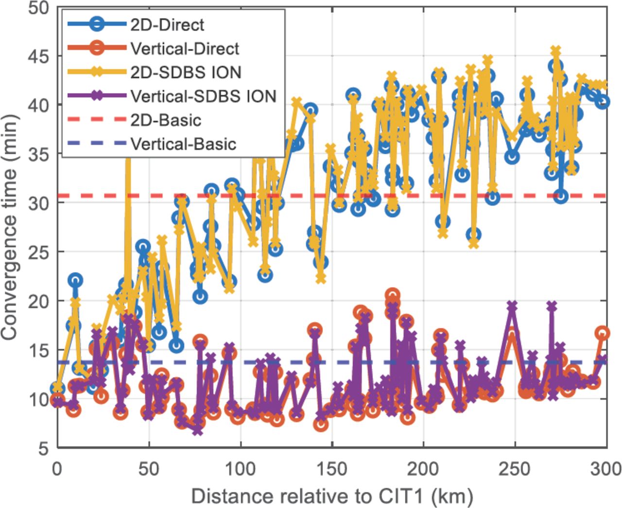
Convergence time to 0.1 m horizontally and 0.2 m at vertical for CIT1 using the direct ionospheric constraints and the SDBS-ION constraints at different distances
The convergence time was reduced to 10 minutes when the reference station was close enough, compared with the convergence time of 31 minutes. When reference stations were more than 100 km away, the convergence time increased. Hence, we believe that inaccurate ionospheric constraints result in biased positioning solutions. Regarding the vertical convergence time, it was generally smaller when adding ionospheric constraints, but it is not the case all the time.
4 DISCUSSION ON IONOSPHERIC CONSTRAINTS
The first concern is how much the precision of ionospheric constraints benefits the PPP convergence. In the basic UPPP model, ionospheric estimates are initialized with the geometry-free combination (P1 – P2). As long as the ionospheric constraints are no less precise than the standard deviation of the geometry-free combination, around  , the ionospheric constraints would be helpful for PPP to converge faster.
Secondly, we investigated the differences in ionospheric constraints between a network and a single station. The previous experiment was carried out based on a single station. The performance of the constraints became less effective as the distance increased. Here we compare the performance using the network solutions. The ionospheric constraints would be more precisely interpolated from a network with better geometry.
We chose a station P589 at 107.7 km with the other two stations of CSST at a distance of 118.2 km and SCIP at 140.5 km, comparing the network solutions with the nearest single station of P589 as presented in Figure 13.

Geographic distribution of a three-station network
Figure 14 shows the performance of positioning using the ionospheric constraints from a single station P589 and a three-station network. The results reveal that the position errors and convergence time both improved using the network solution. The convergence time was also reduced to a 16.4-min average from the 36.6 minutes using a single station of P589. We can see that the interpolated ionospheric constraints from a surrounding network were more accurate than a single station.

Time series of position error at horizontal, vertical, and 3D accuracy of CIT1 using ionospheric constraints from a single station P589 and a three-station network
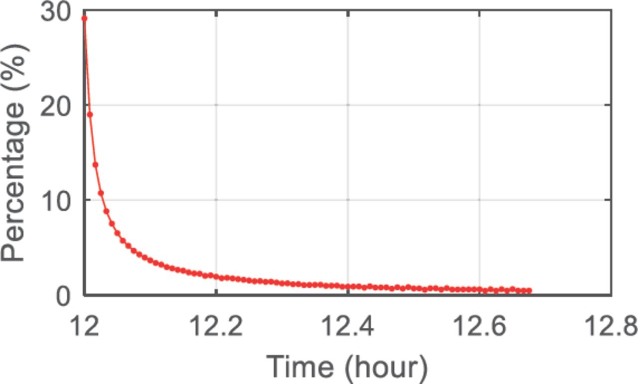
Third, we wanted to explore the question of how the variance of the ionospheric parameter changes after adding ionospheric constraints. We quantified the contribution using the improvement of formal precision. Figure 15 presents the improved percentage of the ionospheric estimate variance with time using data from the example of the reference station AZU1.

Improved percentage of the ionospheric estimate variance against time
It can be observed that the improved percentage drops from 30% to 5% after 10 epochs, which is five minutes. More constraints are less effective when the ionospheric estimates converge to stable values. Therefore, we think the first five-minute ionospheric constraints are beneficial to the PPP convergence for multi-frequency users when the tracking satellites are the same. This information is insightful to users. Downloading or accessing the resources within the first five minutes is good enough.
Finally, it is of interest to note that the correctness and robustness of the ionosphere constraints are significant, especially the ionospheric constraints of the reference satellite. There is a risk that the solutions would deteriorate if the wrong constraints with an unsuitable stochastic model were applied. Here we utilized the formal precision to determine whether the ionospheric observables were applicable. However, as the formal precision becomes smaller, it is restricted to determine whether the ionospheric observables have converged at the right value. Therefore, the quality control of the high precision and robust ionospheric corrections needs further research.
5 CONCLUSION
Instead of applying receiver-biased ionospheric constraints directly, a method of SDBS-ION constraints is developed to eliminate receiver DCBs. The new method, creating single differences of ionospheric corrections with reference satellites, offers a more flexible way to apply ionospheric constraints even without common satellite visibility. Validated by about 130 stations within 300 km, we’ve concluded that the proposed SDBS-ION method yields competitive solutions compared with the method of direct ionospheric constraints.
We also investigated some essential points when adding ionospheric constraints. Results show that the effectiveness of enhancing PPP performance degrades with the increase of the distance between users and reference stations. The positioning errors could be biased when ionospheric constraints are inaccurate. Besides, the ionospheric constraints using the network are more effective when compared with a single reference station. We also found that only the first five-minute ionospheric constraints are beneficial to the PPP when state vectors remain the same.
It is noted that the experiment was implemented under quiet ionospheric conditions; the empirical value of 0.61 mm/km was applied to adjust the stochastic model. The value could be different depending on ionospheric conditions. More accurate and robust ionospheric corrections, which is of great importance to the ionospheric constrained PPP model, merit further research.
HOW TO CITE THIS ARTICLE
Xiang, Y., Chen, X., Pei, L., Luo, Y., Gao, Y., & Yu, W. (2022) On enhanced PPP with single difference between-satellite ionospheric constraints. NAVIGATION, 69(1). https://doi.org/10.33012/navi.505
AUTHORS CONTRIBUTIONS
Yan Xiang designed the research, processed data, and prepared the paper draft; Xin Chen and Ling Pei contributed to the data analysis and revised the manuscript; Yiran Luo contributed to the data analysis; Yang Gao revised the manuscript; and Wenxian Yu supervised the research.
DATA AVAILABILITY
Data and products are downloaded from the Center for Orbit Determination in Europe (CODE), National Oceanic and Atmospheric Administration (NOAA), and the Crustal Dynamics Data Information System (CDDIS). The CORS data are available on the website (https://geodesy.noaa.gov/corsdata).
ACKNOWLEDGMENTS
Products downloaded from CODE and observation data from the US continuously operating reference stations (CORS) are gratefully acknowledged. The study is supported by the Shanghai Pujiang Program of No. 20PJ1409200.
- Received September 6, 2020.
- Revision received September 28, 2021.
- Accepted November 7, 2021.
- © 2022 Institute of Navigation
This is an open access article under the terms of the Creative Commons Attribution License, which permits use, distribution and reproduction in any medium, provided the original work is properly cited.


Jump to section
Related Articles
Cited By...
- No citing articles found.